Orthosteric Drug Effects
Outline
Bi-Molecular Systems51
New Terminology52
What is Drug Antagonism?53
Antagonist Potency53
Mechanism(s) of Receptor Antagonism54
Orthosteric (Competitive and Non-Competitive) Antagonism56
Slow Dissociation Kinetics and Non-Competitive Antagonism62
Partial and Inverse Agonists67
Antagonist Effects In Vivo73
Descriptive Pharmacology: IV74
Summary79
This chapter deals with the quantification of the effects of antagonists to yield empirical measures of antagonist potency. Beginning with the premise that there are two possible modes of action of antagonism; orthosteric blockade (occlusion of the agonist binding site) and allosteric modulation, this chapter focuses on orthosteric antagonism. Estimates of antagonist potency can be obtained for all modes of antagonism through a pA2 value and/or a pIC50 of antagonism of a fixed agonist effect. Patterns of antagonism are then discussed from the standpoint of using these to identify the mechanism of antagonist action (for example orthosteric antagonists producing steric hindrance of agonists). The chapter then discusses how these mechanisms can be used to identify the appropriate mathematical analysis to yield estimates of true system-independent antagonist potency that transcend cell type and measuring system.
Keywords
allosteric, competitive antagonism, hemi-equilibrium, non-competitive antagonism, orthosteric, Schild analysis, surmountable and insurmountable antagonism.
Bi-Molecular Systems
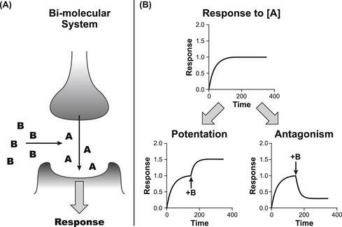
The previous chapters discussed the binding of a molecule to a protein target to cause a change in cellular function (agonism); in these cases the system consists of a single molecule interacting with a target on the cell. There are a large number of pharmacologically relevant interactions that involve two molecules; one causing a change of cellular function and the other interfering with that action. For example, Fig. 4.1 shows a synaptic cleft where a neurotransmitter molecule A is released from the neuron to act on the post-synaptic membrane containing receptors for that neurotransmitter; molecule B can be added to the system to modify the interaction of A with the target. There are two pharmacologically relevant outcomes, namely that the response to A can be increased or diminished (see Fig. 4.1). If the response is increased this could be due to an interference in the disposition of A in the synaptic cleft (inhibition of transport) or allosteric alteration of the target to increase responsiveness. This latter topic will be discussed in Chapter 5. This present chapter discusses the inhibition of the response to A. Implicit in this discussion is the understanding that the effects seen are specific for the drug target being considered, i.e., the molecule does not produce non-specific toxic or other effects on the cell system to modify the cell sensitivity to the agonist.
New Terminology
The following new terms will be introduced in this chapter:
• Allosteric: Describing an interaction mediated by the binding of a molecule to a protein at a distinct site to affect the interaction of that protein with another molecule binding at a different site.
• Antagonism: The process of inhibition of an agonist-driven cellular response by another molecule.
• Competitive antagonism: A specific model of receptor antagonism whereby two molecules compete for a single binding site on the receptor, and the kinetics of binding of both the agonist and antagonist are rapid enough to allow mass action to control the relative proportions of receptor bound to agonist and antagonist.
• Hemi-equilibrium: A condition where there is an insufficient amount of time for complete re-equilibration of agonist and antagonist for a population of receptors according to mass action. This results in a selectively non-competitive effect at high agonist receptor occupancies, causing a partial depression of the maximal response to the agonist.
• Insurmountable: Describing a pattern of agonist dose–response curves whereby the maximal response to the agonist is depressed.
• Non-competitive: Describing antagonism resulting from a system whereby the antagonist does not dissociate from the receptor rapidly enough to allow competition with the agonist.
• Orthosteric: A steric interaction whereby molecules compete for binding at the same site on a protein.
• pA2: Minus logarithm of the molar concentration of an antagonist that produces a two-fold shift of the agonist dose–response curve.
• pIC50: Minus logarithm of the molar concentration of antagonist that produces a 50% inhibition of a defined agonist effect.
• pKB: Minus logarithm of the equilibrium dissociation constant of the antagonist–receptor complex.
• Schild analysis: The application of the Schild equation to a set of dextral displacements produced by a surmountable antagonist; if the Schild plot is linear with a slope of unity the antagonism fulfills criteria for simple competitive antagonism.
• Surmountable: Describing antagonism whereby the agonist dose–response curve is shifted to the right with increasing addition of antagonist, but where the maximal response is not altered.
What is Drug Antagonism?
This chapter will deal with molecules that bind to the target without themselves causing a change (or producing relatively little change), but do interfere with agonists producing response; this is the process of antagonism. There are many therapeutically relevant conditions where an antagonist would be useful, as in cases of inappropriate, excessive or persistent agonism (i.e., inflammation, gastric ulcer) or diseases where remodeling of systems leads to normal agonism becoming harmful (cardiovascular disease). Conceptually, antagonism could be envisioned as the binding of the antagonist to a target to hinder the binding or function (or both) of an agonist. There are three factors that control the extent of antagonism:
• the quantity of antagonist bound (potency);
• the location of the binding relative to the binding of the natural agonist (mechanism);
• the persistence of antagonist binding (antagonist kinetics).
It is worth considering each of these important factors when discussing therapeutically relevant antagonism.
Antagonist Potency
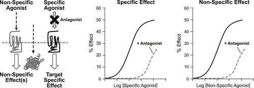
Potency refers to the amount of antagonism in a system for a given concentration of antagonist. The relevant parameter for this is the affinity of the antagonist for the protein target (as defined by Langmuir adsorption binding isotherm; see equation 2.1). Unlike agonism, estimates of antagonist potency should not be cell-type dependent, and thus these are chemical terms that can be measured in a test system and the result applied to all systems, including the therapeutic one. The affinity of an antagonist, quantified as the equilibrium dissociation constant of the antagonist–protein complex, can be measured in an appropriate in vitro system either directly (if a means to trace the protein-bound antagonist species can be quantified, such as in radiolabeled binding assays) or indirectly through interference of agonist activity in a functional assay. This latter approach is preferable as it is what the antagonist will do in vivo that is important. In addition, there are numerous cases where physical binding of molecules and their effect on physiological responses can differ. The desired parameter in this case is referred to as the pKB, namely the negative logarithm of the equilibrium dissociation constant of the antagonist–protein complex. To measure antagonist potency in an in vitro functional assay, comparisons are made between the dose–response curve of the agonist produced in the absence of antagonist, and then again in the presence of antagonist (usually for a range of antagonist concentrations). The resulting pattern of curves is then utilized in an appropriate model defined by the proposed mechanism of action of the antagonist. It should be noted that the antagonism must be shown to be specific for the biological target in question (see Fig. 4.2); it will be assumed that the observed antagonist effects are specific for the target.
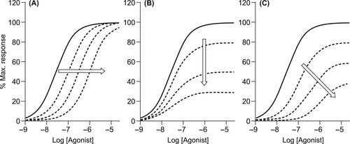
There are two effects an antagonist can have on the dose–response curve to an agonist: depression of maximal response and dextral displacement of the curve (or both; see Fig. 4.3). Both of these effects reflect a diminution of the sensitivity of the system to the agonist in the presence of the antagonist, thus higher concentrations of agonist are required to produce a response in the presence of the antagonist. Different mechanisms of antagonism can produce varying amounts of shift and depression of maxima of the dose–response curves. This can also vary with the type of agonist used to produce response and the sensitivity of the functional system used to measure the effect. For this reason, the pattern(s) of antagonism seen in vitro cannot reliably be used to identify the mechanism of action; in fact, the reverse is true. Once a mechanism of action is identified, then the appropriate model is applied to the data to characterize antagonist potency (pKB values).
Mechanism(s) of Receptor Antagonism
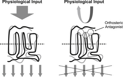
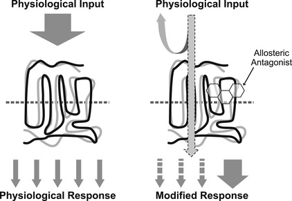
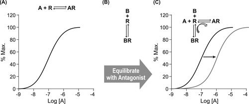
There are two molecular mechanisms operable for the antagonism of responses to endogenous hormones, neurotransmitters or autacoids: orthosteric or allosteric binding. Orthosteric antagonism (see Fig. 4.4) is where the antagonist binds to the same site as the endogenous agonist and precludes agonist binding to the protein. This mechanism is pre-emptive, in that occupancy of the site by the antagonist prevents all actions of the agonist. The second mechanism (allosteric; see Fig. 4.5) is where the antagonist and agonist bind to separate binding sites on the protein, and the interaction between them occurs through a change in conformation of the protein. This type of mechanism is permissive in that some (or even all) actions of the agonist can still be produced when the antagonist is bound. However, some characteristics of the agonist response are modified, such as potency and/or efficacy. Orthosteric antagonism is the most simple and will be discussed in this present chapter; allosteric mechanisms will be discussed in Chapter 5.
Orthosteric (Competitive and Non-Competitive) Antagonism
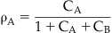
As discussed in Chapter 2, the binding of a molecule to a protein is a stochastic process, meaning that at any one instant there will be a population of protein binding sites where the antagonist is tightly bound to the protein and another where it has momentarily diffused away from the binding site, leaving it open for binding to other molecules. Thus, the probability of another molecule (e.g., agonist) binding to the same site in the presence of the antagonist will be determined by the amount of time the antagonist is momentarily not bound to the protein (determined in turn by the affinity and concentration of the antagonist), and the concentration and affinity of the agonist. Thus it can be seen that in such a system of competition, a very high concentration of agonist theoretically could bind to all of the sites and the maximal response to the agonist would be attained even in the presence of the antagonist. This idea is captured in a simple equation presented by John Gaddum (see Box 4.1), known as the Gaddum equation for competitive kinetics. Specifically, this equation relates the fractional receptor occupancy by a molecule A (ρA) to the concentration A (denoted cA, referring to the concentration normalized as a fraction of the equilibrium dissociation constant of the A–receptor complex), and the normalized concentration of another drug B competing for the same site on the receptor (see Derivations and Proofs, Appendix B5): [1]
Box 4.1
 where ρA is the fractional receptor occupancy by drug A in the presence of another drug B that competes for the binding of A at the receptor. The terms cA and cB refer to the normalized (divided by the equilibrium dissociation constants of the drug–receptor complexes) concentrations of a drugs A and B respectively. It can be seen that if cA >> cB, then the total occupancy of the receptor will revert to a situation identical to that where only molecule A is present, i.e., it will compete with B to the extent that B no longer occupies the receptor.

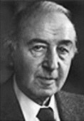
John Henry Gaddum (1900–1965) was a British pharmacologist who did a great deal to propagate quantitative pharmacology. Educated at Cambridge, Gaddum became a medical student at University College London where he applied for, and won, a post at the Wellcome Research Laboratories. There he wrote his first paper on quantitative drug antagonism. After working for the influential pharmacologist Sir Henry Hallet Dale and later chairing the Department of Pharmacology at Cairo University, Gaddum returned to University College London to head the Department of Pharmacology there. At this time, he presented a short communication to the Physiological Society in 1937 entitled “The quantitative effects of antagonistic drugs”[1] which contained the famous “Gaddum equation:”
(4.1)
Therefore, in a completely competitive situation, where the binding of both the antagonist and agonist are rapid, the dose–response curve to the agonist will be shifted to the right in the presence of the competitive antagonist and very high concentrations of agonist will produce the original maximal response (obtained in the absence of antagonist) even in the presence of the antagonist. The shift to the right of the agonist curve reflects the lower probability of the agonist producing a response in the presence of the obstructing antagonist; this probability is increased with increased agonist concentration, therefore the curve reappears at higher concentrations of agonist. The magnitude of the shift in the dose–response curve is proportional to the degree of antagonism and relates to the concentration of antagonist present and its affinity. Schild and colleagues (see Box 4.2) used this fact to devise a method to measure the affinity of competitive antagonists, in a procedure since given the name “Schild analysis” for the construction of a “Schild plot.”[2] The procedure for doing this is shown in Fig. 4.6. The first step is to define the sensitivity of the system to the agonist (obtain a control dose–response curve). Then, the preparation is pre-equilibrated with a defined concentration of the antagonist; this ensures that the receptors and antagonist come to a binding equilibrium according to the Langmuir isotherm. Then, the sensitivity of the tissue is measured again in the presence of the pre-equilibrated antagonist and the shift in the curve is used to estimate the antagonist potency.
Box 4.2
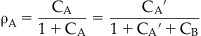
 where pKB is the negative logarithm of the equilibrium dissociation constant of the antagonist–receptor complex; this parameter is a system-independent measure of the potency of a competitive antagonist. An example of this type of analysis is given in Fig. 4.7. It should be noted that for there to be confidence in the veracity of pKB as a true measure of antagonist potency, the Schild plot (line according to equation 4.2) should be linear and have a slope of unity.


Heinz Schild took Gaddum’s equation for competitive binding and ingeniously extended it to provide a tool for the measurement of the potency of a competitive antagonist blocking agonist response. The key to this is the application of the null assumption stating that equal responses to an agonist emanate from equal levels of receptor occupancy by that agonist. This allows the response to a concentration of an agonist A (cA), measured in the absence of an antagonist B, to be represented by ρA. This is the receptor occupancy by A, as given by the Gaddum equation, to be represented (since equal responses are being compared) by the response of the same agonist obtained in the presence of the antagonist:
The concentration of agonist in this latter situation (denoted cA′) will be greater in the presence of the antagonist since it must overcome the competition by antagonist. Cross multiplication and dividing the entire expression by cA results in the Schild equation where cA′/cA is denoted by the equiactive dose–ratio DR:
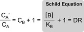 |
For Schild analysis, this is done repeatedly with a range of antagonist concentrations, and then an array of shifts of the control curve produced by a matching array of antagonist concentrations is used to estimate the affinity of the antagonist. The shifts are quantified as ratios of the EC50 of the agonist in the presence and absence of antagonist; these are referred to as dose ratios (DR=EC50[antagonist]/EC50[control]). It can be shown that the log(DR−1) values for a range of concentrations of antagonist [B] have a linear relationship according to the “Schild equation” (see Box 4.2):
(4.2)
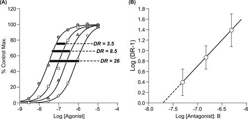 |
| Figure 4.7 Schild analysis. (A) Dose–response curves to the agonist are obtained in the absence and presence of various concentrations of antagonist. The resulting shifts to the right of the agonist dose–response curves are converted to dose ratios (DR) and utilized in the Schild equation (equation 4.2) to construct a Schild regression (shown in panel (B)). Thus, a regression of Log(DR−1) values for a given array of antagonist concentrations provides a linear regression (ideally with a slope of unity) the intercept of which is −pKB. |
Stay updated, free articles. Join our Telegram channel
Full access? Get Clinical Tree
