Additional work by various researchers elucidated the experimental factors that contributed to the proportionality constant k in Equation (5.1) (Brunner and Tolloczko, 1900; Brunner, 1904; Nernst 1904), leading to the form of the Noyes–Whitney equation that is still used today:
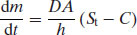
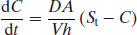
where m is the mass of drug, D is the diffusion coefficient, A is the surface area of dissolving solid, h is the thickness of the unstirred water layer (the boundary layer) surrounding the dissolving solid and C is the concentration of drug in bulk solvent. An alternative version of Equation (5.2) is the Noyes–Whitney–Nernst–Brunner (NWNB) equation, which describes the change in concentration of dissolved solid with time:
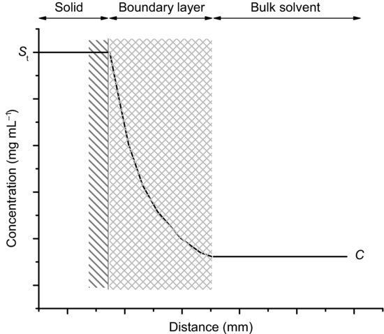
where V is the volume of bulk solvent. In either case, the model assumes that any drug molecule that dissolves at the surface of the solid must then diffuse through a stagnant layer of saturated drug solution surrounding the solid before it moves into the bulk solvent (Figure 5.1). Several other notable models for dissolution have been published, including the interfacial barrier model (Wilderman, 1909) and the Danckwerts’ model (in which a constant stream of macroscopic packets of solvent arrive at the solid surface to absorb solute molecules and transport them to the bulk solvent; Danckwerts, 1951), but the NWNB model is still the model most commonly used.
Figure 5.1 A schematic representation of the boundary layer adjacent to the surface of a dissolving solid and the change in concentration of solute across it.
5.3 Dissolution testing
Concern over the importance of the relationship between the dissolution rate and bioavailability led to the introduction of rotating basket dissolution tests (i.e. a uniform test to measure the dissolution rate in a defined medium) to the US pharmacopoeia in 1970 (although a rotating dissolution method for extended release products was introduced in 1958). In an excellent review of the history of dissolution testing Dokoumetzidis and Macheras (2006) chart the rise in the number of monographs in the US pharmacopoeia that require dissolution tests (Table 5.1). All pharmacopoeias specify dissolution apparatus that should be used for measuring dissolution data (Table 5.2).
Table 5.1 The number of USP monographs for immediate release oral dosage forms requiring dissolution tests (reproduced from Dokoumetzidis and Macheras, Copyright 2006, with permission from Elsevier).
| USP edition/year | Monographs for immediate release dosage forms requiring dissolution testing |
| USP 18-NF 13/1970 | 6 |
| USP 19-NF 14/1975 | 12 |
| USP 20-NF 15/1980 | 60 |
| USP 21-NF 16/1985 | 400 |
| USP 22-NF 17/1990 | 462 |
| USP 23-NF 18/1995 | 501 |
| USP 24-NF 19/2000 | 552 |
| USP 29-NF 20/2000 | 619 |
Table 5.2 Pharmacopoeial dissolution apparatus.
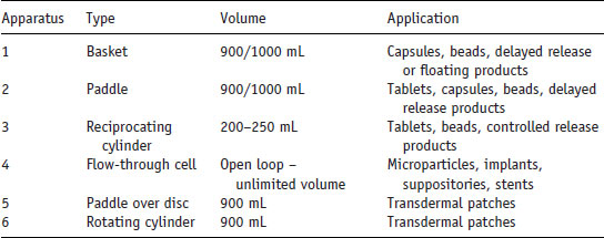
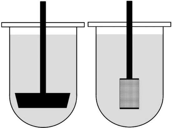
Apparatuses 1 and 2 are similar in arrangement, varying only in the stirrer design (the sample is contained within a rotating basket, apparatus 1, or stirred with a paddle, apparatus 2; Figure 5.2). The dissolution medium (900 or 1000 mL) is contained in a round-bottomed vessel housed in a thermostatted water bath. Both methods allow the pH of the dissolution medium to be changed during the test (although this is slightly easier with apparatus 1 in cases where the drug product is contained within the basket), mimicking the change in pH along the GI tract. One problem with apparatus 2 is that the drug product might float, in which case a ‘sinker’ (typically a small piece of coiled, nonreactive wire) can be attached to the drug product.
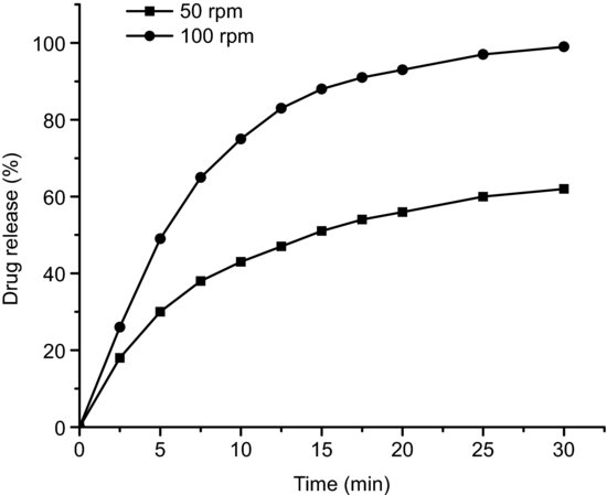
The hydrodynamics of the medium will vary with stirring rate, which may also affect dissolution. In particular, slow stirring speeds in apparatus 2 can lead to a ‘coning’ effect, where the dissolving compact forms a cone at the bottom of the vessel. This effect has been shown to reduce the dissolution rate for immediate release products that contain a large proportion of insoluble excipients or products containing BCS class II or IV poorly soluble drug substances (Klein, 2006). Figure 5.3 shows the dissolution profiles for indomethacin tablets at two stirring speeds where this effect can be seen.
Figure 5.3 Dissolution curves for indomethacin tablets stirred at 50 and 100 rpm (data redrawn from Klein (2006)).
Drug concentrations are most conveniently determined with UV spectrophotometry, either by removing aliquots of solution at regular time intervals, by circulating the dissolution medium through a UV cuvette and taking in-line measurements or by using a fibre-optic UV probe immersed directly in the dissolution vessel, although other assays can be used if the drug substance does not have a suitable UV chromophore.
Study question 5.1 Can you see a potential drawback in removing aliquots of solution for analysis?
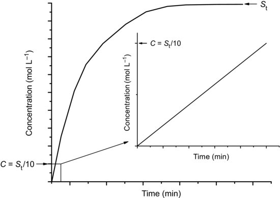
Irrespective of how it is performed, a dissolution test will result in a plot of concentration versus time (Figure 5.4). Equation (5.3) predicts that the rate of change of concentration with time will decrease as the concentration of solute increases; as depicted in Figure 5.4, the rate of dissolution (given by the gradient of the line) starts at a maximum and asymptotically approaches zero as the concentration approaches the solubility. A further complication is that the surface area of the dissolving solid will also change with time (initially there may be a large increase if, for instance, a compact disintegrates, followed by a decrease to zero) and this will affect the dissolution rate. It is thus difficult to define a dissolution rate for a given material since the rate is constantly decreasing. A general convention is to construct dissolution experiments such that the final concentration attainable, if all the material dissolves, is never greater that 10% of the equilibrium solubility. The inset graph of Figure 5.4 shows the dissolution data plotted over this 10% region and it can be seen that the gradient of the line (and hence the dissolution rate) is essentially constant. When constructed in this way the dissolution experiment has been performed under sink conditions.
Figure 5.4 Concentration versus time profile for a solute undergoing dissolution following addition to water and (inset) the linear rate region when C = St//10 (i.e. sink conditions).