(1)
Department of Mathematics, University of Florida, Gainesville, FL, USA
16.1 Single-Species Discrete Population Models
The continuous population models that we have considered in previous chapters model population and epidemic processes that occur continuously in time. In particular, they assume that births and deaths in the population occur continuously. This assumption is true for the human population, but many insect and plant populations have discrete, nonoverlapping generations. Such populations reproduce during specific time intervals of the year. Consequently, population censuses are taken at those specific times. As a result, modeling such populations and the distribution of disease in them should happen at discrete times. In this chapter we introduce discrete single-species population and epidemic models.
16.1.1 Simple Discrete Population Models
We assume that we measure the population at discrete, equally spaced, moments of time:  , and we find that the population numbers at these moments of time are N t , where t takes the values of
  . For simplicity, we will set
  . Thus, the population size is described by a sequence:
  . A discrete population model can be written in the following general form:

where  is a specified function of N n . That is, if we know the population size at time t n , the model tells us what the populations size at time t n+1 should be. Such a model is equipped with a given initial condition: the population size N 0 at time t 0 is given. Another way to rewrite Eq. (16.1) is

The function f(N n ) is called a fitness function or per capita rate of population growth or net reproduction rate.
 , and we find that the population numbers at these moments of time are N t , where t takes the values of
  . For simplicity, we will set
  . Thus, the population size is described by a sequence:
  . A discrete population model can be written in the following general form:
(16.1)
 is a specified function of N n . That is, if we know the population size at time t n , the model tells us what the populations size at time t n+1 should be. Such a model is equipped with a given initial condition: the population size N 0 at time t 0 is given. Another way to rewrite Eq. (16.1) is
(16.2)
Such difference equations are of first order, because they contain only one time step. They are also autonomous, because  does not depend explicitly on the time t n . The simplest discrete population model is derived under the assumption that individuals die with constant probability d. Furthermore, we assume that b individuals are born per individual in the population. The model then becomes
 that is, the number of individuals at the time step t n+1 is the number from the time step t n plus those who have been born, minus those who have died. Defining
  , we obtain the following linear discrete equation of population growth:

The parameter  is called the net reproduction number. We note that
 ![$$ \mathcal{R} > 0 $$
” src=”/wp-content/uploads/2016/11/A304573_1_En_16_Chapter_IEq9.gif”></SPAN>, since <SPAN class=EmphasisTypeItalic>b</SPAN> and <SPAN class=EmphasisTypeItalic>d</SPAN> are probabilities and are less than one. Model (<SPAN class=InternalRef><A href=]() 16.3) is a discrete analogue of the Malthusian equation. Equation (16.3) is a special case of Eq. (16.2) with
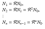
16.3) is a discrete analogue of the Malthusian equation. Equation (16.3) is a special case of Eq. (16.2) with  . Model (16.3) can be solved. Given initial population size N 0, we have
If  , then each individual leaves fewer than one descendant, and the population declines geometrically. If
  , the population remains constant. These model predictions are valid under the assumption that the resources are unlimited.
 does not depend explicitly on the time t n . The simplest discrete population model is derived under the assumption that individuals die with constant probability d. Furthermore, we assume that b individuals are born per individual in the population. The model then becomes
 , we obtain the following linear discrete equation of population growth:
(16.3)
 is called the net reproduction number. We note that
  . Model (16.3) can be solved. Given initial population size N 0, we have
(16.4)
 , then each individual leaves fewer than one descendant, and the population declines geometrically. If
  , the population remains constant. These model predictions are valid under the assumption that the resources are unlimited.
In practice, populations do not experience unlimited growth, so models that predict asymptotically bounded growth are more realistic. One such model is the discrete analogue of the logistic equation. To derive such an analogue, we approximate the continuous time derivative with N n+1 − N n , assuming that the time step is equal to one. Thus the discrete logistic equation takes the form

First we factor N n and r + 1. Furthermore, we make the following changes in dependent variables and parameters:
 We obtain a classical form for the discrete logistic equation:
 This method for producing discrete equations is not foolproof, however. The discrete logistic equation above is not well posed, in the sense that its solutions can become negative. This is not hard to see. Suppose we start from y 0 = 0. 5 and a = 6. Then y 1 = 1. 5. Consequently, y 2 < 0. Thus, the logistic equation is not a very good discrete population model.

(16.5)


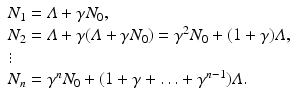
We can derive a discrete version of the simplified logistic model. Suppose the population increases in each time interval by a constant amount  , and that γ ≤ 1 is the probability for survival of individuals to the next time period. Then the simplified logistic model takes the form

This model can also be solved explicitly:
Hence,

 , and that γ ≤ 1 is the probability for survival of individuals to the next time period. Then the simplified logistic model takes the form
(16.6)

(16.7)

(16.8)
Other discrete population models have been proposed that guarantee that the population remains positive for all times. One such model, proposed by Bill Ricker [138], is the Ricker model:


(16.9)
Another model also widely used is the Beverton–Holt model [23], also called the Verhulst equation:


(16.10)
A generalization of the Beverton–Holt model can be made that is known as the Hassell equation [72]:

where b > 0 is a positive parameter.

(16.11)
16.1.2 Analysis of Single-Species Discrete Models
Difference equations also have solutions that do not depend on time, called equilibria. Since the solution does not depend on time, all members of the sequence have the same value, that is, we have
 Consequently, equilibria of the difference equation (16.1) must satisfy
  .
.

 .
.Definition 16.2.
A value N ∗ that satisfies
 is called a fixed point of the function
  .
.

 .
.Example 16.1.
Consider the equilibria of the logistic equation
 The solutions of this equation are N 1 ∗ = 0 and N 2 ∗ = K, that is, the equilibria in the discrete case are exactly the same as in the continuous case. The equilibrium N 1 ∗ = 0 is called a trivial equilibrium, while the equilibrium N 2 ∗ = K is called a nontrivial equilibrium.

To describe the behavior of the solutions near an equilibrium, we use again a process called linearization. Let N ∗ be the equilibrium, and u n the perturbation of the solution from the equilibrium, that is,
 Substituting this equation into Eq. (16.1), we have
  . Expanding
  in a Taylor series and neglecting all terms containing powers of u n greater than one, we obtain
 Recall that since N ∗ is an equilibrium, we have
  . Hence, we obtain the following linearized equation:

We note that  is a fixed number, which may be positive or negative. If we consider


 . Expanding
  in a Taylor series and neglecting all terms containing powers of u n greater than one, we obtain
 . Hence, we obtain the following linearized equation:
(16.12)
 is a fixed number, which may be positive or negative. If we consider
(16.13)
then Eq. (16.13) is exactly the discrete Malthus equation. Consequently, we have the following:
1.
If  , then u n → 0. Hence, N n − N ∗ → 0 and N n → N ∗. This is the case if N 0 is close enough to N ∗, that is, this result is local. In this case, we call N ∗ locally asymptotically stable.
 , then u n → 0. Hence, N n − N ∗ → 0 and N n → N ∗. This is the case if N 0 is close enough to N ∗, that is, this result is local. In this case, we call N ∗ locally asymptotically stable.
2.
If  . Hence
  , and N n diverges from N ∗. This is the case if N 0 is close enough to N ∗. In this case, we call N ∗ unstable.
 . Hence
  , and N n diverges from N ∗. This is the case if N 0 is close enough to N ∗. In this case, we call N ∗ unstable.
We note that if  , we cannot draw conclusions from the local analysis.
 , we cannot draw conclusions from the local analysis.
We summarize the above discussion in the following theorem:
Theorem 16.1.
The equilibrium N ∗ of the discrete equation(16.1)is locally asymptotically stable if and only if  . The equilibrium N ∗ of the discrete equation (16.1) is unstable if and only if
 ![$$ \vert \mathcal{F}'(N^{{\ast}})\vert > 1 $$
” src=”/wp-content/uploads/2016/11/A304573_1_En_16_Chapter_IEq27.gif”></SPAN> <SPAN class=EmphasisTypeItalic>.</SPAN> </DIV></DIV><br />
<DIV class=Para>To illustrate the use of the theorem above, we consider the local stability of the equilibria of the logistic equation.</DIV><br />
<DIV id=FPar5 class=]()
 . The equilibrium N ∗ of the discrete equation (16.1) is unstable if and only if
 Example 16.2.
In the case of the logistic equation (16.5), the function  is given by
 The derivative is given by
 In the case of the trivial equilibrium N ∗ = 0, we have
 So if | 1 − r | < 1, or equivalently, if 0 < r < 2, then the nontrivial equilibrium is locally asymptotically stable.
 is given by


When r > 2, simulations suggests that the logistic equation can experience very complex behavior. To investigate this behavior through simulations, we will study the nondimensionalized version of the logistic equation:

Recall that ρ = 1 + r, so we can expect complex behavior for ρ > 3. We notice that the corresponding equilibria of the nondimensional logistic model are y ∗ = 0 and y ∗ = 1. The first complexity that appears is a 2-cycle.

(16.14)
Definition 16.3.
In model (16.14),  . As ρ increases, the system experiences a process, called period-doubling, to a 4-cycle. Similarly, a 4-cycle of model (16.14) is a system of four solutions y 1, y 2, y 2, y 4 such that

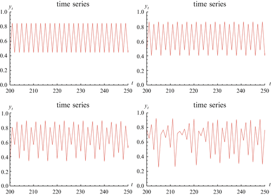
Further period-doubling occurs to an 8-cycle. The period-doubling continues until the system begins to exhibit chaos. We illustrate period-doubling and chaos in Fig. 16.1.
 . As ρ increases, the system experiences a process, called period-doubling, to a 4-cycle. Similarly, a 4-cycle of model (16.14) is a system of four solutions y 1, y 2, y 2, y 4 such that
(16.16)

Fig. 16.1
The figure shows time series of the model y n+1 = ρ y n (1 − y n ) for different values of ρ. The first figure shows a two-cycle with ρ = 3. 43. The second figure on the top line shows a 4-cycle with ρ = 3. 47. The left figure on the bottom row shows an 8-cycle with ρ = 3. 58. The right figure on the bottom row shows chaos with ρ = 3. 7
16.2 Discrete Epidemic Models
Just like single-species population models, discrete epidemic models can also be obtained from a discretization of the continuous epidemic models. However, this approach results in models that have issues like those of the discrete logistic equation. To avoid these problems, a modeling approach specific to discrete models should be taken. We follow here the approach of Castillo-Chavez and Yakubu [39].
16.2.1 A Discrete SIS Epidemic Model
We begin with a general population model

where γ < 1 is the probability of survival to the next time period, and f(N n ) is a recruitment function. We assume that the disease does not affect the population dynamics, that is, we assume that the disease is nonfatal and does not affect the birth process. We will build an SIS epidemic process on top of the demographic process. We denote by S n and I n the susceptible and infected individuals at time t n . Individuals survive with probability γ < 1 (die with probability 1 −γ) in each generation. Infected individuals recover with probability  (do not recover with probability
  ) in each generation. In each generation, susceptible individuals become infected with probability 1 − G (remain susceptible with probability G). The function G is a function of the prevalence I n ∕N n , which is weighted with coefficient α. The model assumes a sequential process: at each generation, γ S n susceptibles survive, and the surviving susceptibles become infected with probability 1 − G. Similarly, γ I n infected individuals survive, and the surviving ones recover with probability
  :
:

The function G must satisfy the following conditions:

(16.17)
 (do not recover with probability
  ) in each generation. In each generation, susceptible individuals become infected with probability 1 − G (remain susceptible with probability G). The function G is a function of the prevalence I n ∕N n , which is weighted with coefficient α. The model assumes a sequential process: at each generation, γ S n susceptibles survive, and the surviving susceptibles become infected with probability 1 − G. Similarly, γ I n infected individuals survive, and the surviving ones recover with probability
  :
:
(16.18)
1.
![$$ G: [0,\infty ) \rightarrow [0,1] $$](/wp-content/uploads/2016/11/A304573_1_En_16_Chapter_IEq33.gif) .
.
![$$ G: [0,\infty ) \rightarrow [0,1] $$](/wp-content/uploads/2016/11/A304573_1_En_16_Chapter_IEq33.gif) .
.2.
G(0) = 1.
3.
G is a monotone decreasing function with G′(x) < 0 and G″(x) ≥ 0.
16.2.2 Analysis of Multidimensional Discrete Models
In this subsection, we introduce the techniques that help us analyze systems of discrete equations. Suppose that we are given the following system:

where x is an M-dimensional vector of variables. As before, an equilibrium of system (16.19) is the solution of the problem
 To find the behavior of the solutions near an equilibrium, we use linearization. We set x n = u n +x ∗. We obtain the following linear system:

where J is the Jacobian of the system, that is,


(16.19)


(16.20)

(16.21)
Definition 16.4.
An equilibrium point x ∗ is said to be locally asymptotically stable if there exists a neighborhood U of x ∗ such that for each starting value x 0 ∈ U, we get

The equilibrium point x ∗ is called unstable if x ∗ is not (locally asymptotically) stable.

(16.22)
The limit (16.22) holds if for system (16.20), we have  . The following theorem gives the conditions for convergence of solutions of the linear system (16.20) to zero:
 . The following theorem gives the conditions for convergence of solutions of the linear system (16.20) to zero:
Theorem 16.2.
Let J be an M × M matrix with ρ( J ) < 1, where
 Then every solution of ( 16.20 ) satisfies
 If ρ( J ) > 1, then there are solutions that go to infinity.


This implies the following criterion for stability of an equilibrium x ∗ of system (16.19).
Theorem 16.3.
Consider the nonlinear autonomous system ( 16.19 ). Suppose  , where
  and
and  is an open set. Suppose
  is twice continuously differentiable in some neighborhood of a fixed point
  . Let J ( x ∗ ) be the Jacobian matrix of
  evaluated at x ∗ . Then the following hold:
 , where
  and
and  is an open set. Suppose
  is twice continuously differentiable in some neighborhood of a fixed point
  . Let J ( x ∗ ) be the Jacobian matrix of
  evaluated at x ∗ . Then the following hold:
1.
x ∗ is locally asymptotically stable if all eigenvalues of J ( x ∗ ) have magnitude less than one.
2.
x ∗ is unstable if at least one eigenvalue of J ( x ∗ ) has magnitude greater than one.
The Routh–Hurwitz criterion will not be helpful here in determining which matrices are stable, since Routh–Hurwitz identifies matrices whose eigenvalues lie in the left half of the complex plane. However, there is an analogous criterion that can help determine whether the spectral radius of a matrix is smaller than one. This criterion is called the Jury conditions. Let
 where a M = 1. To introduce the Jury conditions, we first have to introduce the Jury array. The Jury array is composed as follows: First we write out a row of the coefficients, and then we write out another row with the same coefficients in reverse order. The first two rows of the Jury array are composed of the coefficients of the polynomial
  above. Once we have the first two rows of the a coefficients, the next two rows are of the b coefficients, and so on. We obtain the array of Table 16.1, where the b coefficients, c coefficients, etc., are composed as follows:

 above. Once we have the first two rows of the a coefficients, the next two rows are of the b coefficients, and so on. We obtain the array of Table 16.1, where the b coefficients, c coefficients, etc., are composed as follows:
Table 16.1
Jury array
Number | Coeff. | Coeff. | Coeff. | Coeff. | Coeff. |
|---|---|---|---|---|---|
(1) | a 0 | a 1 | … | a M−1 | a M |
(2) | a M | a M−1 | … | a 1 | a 0 |
(3) | b 0 | b 1 | … | b M−1 | |
(4)
Stay updated, free articles. Join our Telegram channel
Full access? Get Clinical Tree
 Get Clinical Tree app for offline access

|
