which is roughly the size of a cell. The domain contains blood vessels which are the sources of oxygen and nutrients. In our previous work the 2D micro-vasculature was generated using a diffusion CA model [9]. In this work we used a constrained constructive optimization (CCO) algorithm to grow the vascular network. This powerful algorithm has been used to simulate vascular network in 2D [10] and also in 3D [11]. The full description of the CCO algorithm is not provided here, but an interested reader can find more information from literature [10, 11].
In brief, the CCO algorithm grows trees in a manner that fulfils the principle of minimum blood volume, i.e., only a minimum necessary amount of blood is required to perfuse a tissue/organ. Practically an input mean flow rate and a global pressure drop need to be defined for the tree. Figure 1 shows a 3D vasculature of 2,000 vessels, with the flow rate at the root vessel being 1. 0 × 10−3 ml and the pressure drop being 5 mmHg across the tree. This vasculature will be used in the 3D domain for oxygen diffusion simulation.
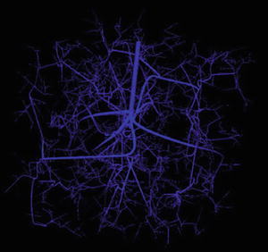

Fig. 1
Micro-vasculature generated using CCO algorithm
2.2 Oxygen Distribution
The transient diffusion equation in 3D can be expressed as [12]:

where
is the diffusion coefficient [12],
is the magnitude of oxygen concentration in the whole domain at location
and time t. With a finite difference method explicit in time (n) and centered in space (i, j, k) and without considering the oxygen consumption term k, Eq. (1) becomes:


(1)


(2)
As the spatial step was fixed (10 μm), step time has to be chosen to obtain a stable scheme for diffusion. Thus, stability conditions are given by the diffusion number
, which gives us:
and therefore Δ t = 1 ms was chosen.


A significant difference between the 2D and 3D versions of oxygen diffusion was that the computer memory for the matrix size needs to be considered, especially when floating numbers (default as the data type 64-bit double) are used for the representation of C values for the lattice. In order to reduce the computational cost, the matrix vectorization was used where the concentration at each coordinate C(i, j, k) was identified with an index l and so:


(3)
The internal computation will be made with index l but the result interpretation will be made with indexes i, j, k. A new matrix A was created which will be the basis of the computation and a standard line for A is:
![$$\displaystyle{ \begin{array}{l} A(l,:) = [C(i,j,k)C(i - 1,j,k)C(i + 1,j,k)C(i,j - 1,k) \\ \qquad \qquad C(i,j + 1,k)C(i,j,k - 1)C(i,j,k + 1)]\end{array} }$$](/wp-content/uploads/2016/10/A321864_1_En_3_Chapter_Equ4.gif)
(4)
This vectorization scheme resulted in significantly improved computation time. For example, it took around 1 h to compute the first iteration in a conventional matrix form in Matlab. With vectorization it computes much faster: about 60 s for 100 iterations, while saving all the data in a 4D-matrix (three coordinates for space and the last one for time). Without saving the data the computation time for 1,000 iterations was about 450 s.
2.3 Cellular Automata Domain and Rules
To enable cancerous/normal cells to evolve in the 3D domain, we need to define CA rules. The first rules were adapted from Alarcon et al. [1]. In brief, a cancerous cell is similar to normal cells in that it may only proliferate if oxygen is present in that element. However a cancerous cell can survive and also enter a quiescent state when no oxygen is present in that element. Once a cancerous cell enters a quiescent state, a clock is started and the cell’s functions are suspended, including proliferation. The clock is incremented at each time step if no oxygen is present in that centre element. The cell dies once the clock reaches a certain value. However, if oxygen enters the cell at any time, it returns to proliferation state and the clock is reset to zero. The CA model was run on a Neumann lattice, which in three dimensions results in six nearest neighbours (Fig. 2).


Fig. 2
Neumann neighborhood in 3D: each element has six neighbour elements
Initial proportions of normal and cancer cells in the domain were arranged as 70–30, i.e. more normal cells than cancer cells to enable the development of a normal cell colony. No difference of behaviour between cancer cells and normal cells was considered except the competition rules, which were:
1.
If a free element is surrounded by more normal cells than cancerous cells, it would become a normal cell only if there is enough oxygen for the cell to spread into the free element.
2.
If a free element is surrounded by an equal number of normal and cancer cells, it would become a cancerous cell, if there is enough oxygen for the cell to spread into the free element.
The above simple rules, when coupled with the diffusion equation, enabled us to simulate different cell growth patterns, as described in Sect. 3.
3 Results
3.1 Oxygen Diffusion in the 3D Domain
The oxygen diffusion based on Eq. (1) and the vasculature of Fig. 1 were solved with the initial condition C = 0 kg-mol everywhere in the domain. Figure 3 shows the oxygen distribution isosurfaces when the solution became steady. The concentration gradient from the vasculature to the tissue can be seen from the four isosurfaces in the figure.


Fig. 3
Isosurfaces of different oxygen concentrations
With an oxygen distribution in the background, the cancer and normal cells may survive and compete with each other. The different growth patterns presented below include:
the colony at the end of a simulation: cancer cells in red, normal cells in green and vessels in blue
the evolution of the number of cells during the simulation
the parameters used in the simulation (diffusion coefficient D and uptake ratio k)
3.2 Cancer/Normal Cell Competition Under Hypoxia
Firstly we considered the scenario where there was an insufficient oxygen supply due to a disrupted vascular network, or the uptake in tumour cells greatly exceeded the supply of the host tissue. We simulated an acute case where a colony started from a normal oxygen concentration distribution shown in Fig. 3, but the oxygen concentration diminished with time due to consumptions from cells. Because of the competition law and the difference of oxygen concentrations needed for proliferation, cancer cells resisted hypoxia better than normal cells.
It can be seen in Fig. 4 that since there was no supply of oxygen from the vessels, the colony decreased and once the oxygen was totally consumed, the cells disappeared. However, under the same initial condition but with different oxygen consumption rates between cancer and normal cell, the initialization enabled normal cell to spread further than cancer cells. However, in the end there were still more cancer cells than normal cells before the disappearance of the colony (Fig. 5).


Fig. 4
Hypoxia state simulation. Concentration needed to spread into cells: C normal = 0. 03 kg m−3,
. Oxygen consumption rate:
,


Fig. 5
Hypoxia state simulation. Concentration needed to spread into cells: C normal = 0. 03 kg m−3,
. Oxygen consumption rate:
,


3.3 Cancer/Normal Cell Competition Under Steady Oxygen Supply Conditions
We considered another scenario where the vasculature was effectively functioning and the colony received constant oxygen supply. Since the difference remained only in the consumption rates and the initialization was still favourable for normal cells, the normal cells stayed more numerous than cancer cells until the colonies were stable (Fig. 6).


Fig. 6
Oxygenated state simulation. Concentration needed to spread into cells: C normal = 0. 02 kg m−3,
. Oxygen consumption rate:
,


Lastly we ran another simulation where the cancer cell growth was strongly favoured due to a much lower concentration needed to spread into adjacent cells, and also a lower uptake rate (Fig. 7). However, the colony of normal cells displayed a resistance to cancer cells in that it remained in the domain. Also note that the tumour cells did not propagate across the whole domain due to low oxygen concentrations in areas far from vessels. Indeed, Folkman observed that tumour cells at a distance of more than 150 μm from capillaries were transformed into necrosis cells [13].


Fig. 7
Oxygenated state simulation. Concentration needed to spread into cells:
,
. Oxygen consumption rate:
,


4 Discussion
It is well known that a compact solid tumour will grow to a diffusion-limited size, after which it will have to recruit existing vasculature, or acquire a new one through angiogenesis in order to grow further [8, 13]. In the process of metastasis the role of a vascular network is also crucial. In this project we adopted a highly complex 3D vasculature as the source for oxygen diffusion. The goal was to study the growth pattern of a 3D colony of competing normal and cancerous cells by the means of CA, with varying oxygen diffusion and uptake rates occurring at the background. Through the implementation and adjusting of a set of CA rules, evolution of the colony was visualized and compared.
The assumptions of the simulations were rather idealistic. Firstly, angiogenesis happened separately from metastasis and so the vasculature was created before the computation; secondly, the initialization was from a random colony of 25 cells (70 % of normal cells and 30 % of cancer cells), located in the centre of the vasculature; Thirdly, the growth coefficient was empirically configured. Future works include incorporation of a vasculature network that would evolve with, and due to, the tissue would greatly increase validity. More specifically, vasculature that responds to growth factors emitted by cancerous tissue would be included.
The spatial scale (1 mm) of the current hybrid CA-continuum model provides an excellent interface for multiscale modelling. Moreover, the current domain configuration ( × 106 cells of ∼ 1 mm in each dimension) represents the size of some fundamental units of biosystems, e.g., the liver lobule, which has a complex vessel organization. Thus the current framework represents our first effort for ensuing 3D vasculature-based tumour growth models. For example, from a computational perspective it is possible to incorporate more complex CA rules. One of such rules is to allow a cancer cell to divide even when there is no free space around it—the tumour cell mitosis scheme as introduced in [6].
5 Conclusion
In this paper we presented a hybrid CA-continuum method to simulate cancer and normal cell competition in a 3D domain with a complex vasculature. The current work established a flexible framework to incorporate more realistic CA rules and diffusion/uptake parameters.
Acknowledgement
We thank Mr. Alexandre Muller for his help in the tree growing CCO algorithm.
References
1.
Alarcon, T., Byrne, H., Maini, P.: A cellular automaton model for tumour growth in inhomogeneous environment. J. Theor. Biol. 225(2), 257–274 (2003)CrossRefMathSciNet
2.
3.
Chopard, B., Droz, M.: Cellular Automata Modeling of Physical Systems. Springer, New York (2012)CrossRef
4.
Moreira, J., Deutsch, A.: Cellular automaton models of tumor development: a critical review. Adv. Complex Syst. 05(02n03), 247–267 (2002)
5.
Byrne, H.M., Alarcon, T., Owen, M.R., Webb, S.D., Maini, P.K.: Modelling aspects of cancer dynamics: a review. Philos. Trans. R. Soc. A: Math. Phys. Eng. Sci. 364(1843), 1563–1578 (2006)CrossRefMathSciNet
6.
Düchting, W., Vogelsaenger, T.: Recent progress in modelling and simulation of three-dimensional tumor growth and treatment. Biosystems 18(1), 79–91 (1985)CrossRef
7.
Kansal, A.R., Torquato, S., Harsh, G.R., Chiocca, E.A., Deisboeck, T.S.: Simulated brain tumor growth dynamics using a three-dimensional cellular automaton. J. Theor. Biol. 203(4), 367–382 (2000)CrossRef
8.
Wise, S.M., Lowengrub, J.S., Frieboes, H.B., Cristini, V.: Three-dimensional multispecies nonlinear tumor growth – i: model and numerical method. J. Theor. Biol. 253(3), 524–543 (2008)CrossRefMathSciNet
9.
Deacon, N., Chapuis, A., Ho, H., Clarke, R.: Modelling the tumour growth along a complex vasculature using cellular automata. In: Computational Biomechanics for Medicine. Springer, Berlin (2014)CrossRef
10.
Schreiner, W., Buxbaum, P.: Computer-optimization of vascular trees. IEEE Trans. Biomed. Eng. 40(5), 482–491 (1993)CrossRef
11.
Karch, R., Neumann, F., Neumann, M., Schreiner, W.: A three-dimensional model for arterial tree representation, generated by constrained constructive optimization. Comput. Biol. Med. 29(1), 19–38 (1999)CrossRef
12.
Shrestha, S.M.B., Joldes, G.R., Wittek, A., Miller, K.: Cellular automata coupled with steady-state nutrient solution permit simulation of large-scale growth of tumours. Int. J. Numer. Methods Biomed. Eng. 29(4), 542–559 (2013)CrossRef
13.
Folkman, J.: Angiogenesis in cancer, vascular, rheumatoid and other disease. Nat. Med. 1(1), 27–30 (1995)CrossRef

Stay updated, free articles. Join our Telegram channel

Full access? Get Clinical Tree

