Summarizing Evidence for Medical Practice
Comparative Effectiveness 11
HEALTH SCENARIO
Dr. Block was just told by his nurse that Mr. Green had been “squeezed” into his schedule at lunchtime tomorrow. This is Mr. Green’s fifth visit in 9 weeks. Mr. Green is a 54-year-old high school football coach who is being treated for major depression. His wife called, very upset, to make the appointment and told the nurse that “his medicine is just not working, and he is really bad.” Mr. Green has tried two different types of antidepressant drugs before the currently prescribed medication. One was changed after 14 days because of intolerable side effects, and the second was changed after 3 weeks because of a combination of side effects and lack of improvement. Dr. Block reviewed Mr. Green’s record and pondered what to do next. During a previous discussion about potential treatment options, Mr. Green said that he does not believe in counseling because “he tried it when he lived in Michigan and it does not work.”
Dr. Block must consider the advantages and disadvantages of the available treatment options for this patient: (1) switch to another antidepressant, (2) augment the current antidepressant with a second agent, (3) try to persuade the patient to get counseling in addition to medication, (4) consider electroconvulsive therapy (ECT), or (5) refer him for repeated transcranial magnetic stimulation (r-TMS) treatment. What to do? Then he remembers having seen some recent reports on advances in depression treatment, and he decides to search for evidence on the comparative effectiveness (CE) of the approaches that he is considering for Mr. Green.
To find a summary of the evidence, he first searches the website of the Agency for Healthcare Research and Quality (AHRQ). He finds a list of Clinician Research Summaries, including one on “Non-pharmacologic Interventions for Treatment-Resistant Depression in Adults” (AHRQ Clinician Research Summaries, 2012). Great, he thinks, my problem is solved. That is until he sees that the summary identifies a number of important gaps in the knowledge in the studies reviewed, including (1) information on quality of life is substantially missing from the studies; (2) few studies compare nonpharmacologic interventions with each other or with pharmacologic interventions or combinations of treatments; (3) there is almost no evidence on how the CE might differ for patient subgroups defined by age or sex; and (4) the studies use inconsistent measures of treatment resistance, clinical outcomes, and adverse events and have short follow-up periods.
When he retrieves the full research report (www.effectivehealthcare.ahrq.gov/trd.cfm), he finds that most of the studies were published before 2008 and thus are 6 or more years old and not clearly relevant to his current patient. Shaking his head at the clear lack of external validity and relevance of these studies to his clinical problem, he gives up and decides he will have to spend some time doing more detailed searches for evidence tonight after dinner.
This physician is a problem solver who is approaching the practice of medicine from the perspective of patient-centered care. He knows that different treatments may work differently in different patients and that the most efficacious treatment for a cohort of patients in a clinical trial may not be the most effective or acceptable therapy for a specific patient. He needs quick information on the CE of the therapies that he thinks will be acceptable to his patient. This very real practice need is the reason for the current focus on comparative effectiveness research (CER).
COMPARATIVE EFFECTIVENESS RESEARCH
The Congressional Budget Office (CBO, 2007) defined CER as: “rigorous evaluation of the impact of different options that are available for treating a given medical condition for a particular set of patients” (CBO, 2007 p. 3). A report from the Institute of Medicine (IOM, 2009) that lists CER topics that should be top priorities for funding also identifies four types of research designs that are relevant for CER: (1) systematic reviews and meta-analyses, (2) decision analysis models, (3) observational studies (OSs), and (4) large pragmatic clinical trials.
Performing a systematic review, using a decision analysis model, or analyzing observational data from his own patients or from a large health systems database is clearly not feasible for informing Dr. Block’s treatment decisions in the Health Scenario. Furthermore, he knows that these methodological approaches do not provide the level of evidence that would result from a well-designed and executed randomized controlled trial (RCT). It would be ideal if he could find the results of a large pragmatic clinical trial that compared his five treatment choices for middle-aged men who have failed two previous pharmaceutical treatments for depression and who have a history indicating that counseling for depression is not effective. However, such a trial does not exist. Indeed, it may be impossible and unethical to do such a trial because there is substantial evidence available from individual studies to indicate that ECT (Nahas et al., 2013) and r-TMS (Carpenter et al., 2012) are effective in a majority of patients with treatment-resistant depression and that augmentation of antidepressants with additional drugs has only a moderate effect in patients with a history of previous drug failures (Fava et al., 2006). Thus, because Dr. Block will have to rely on reports of effectiveness of treatments that do not use the strongest possible research design to ensure the internal validity of findings and thus may be affected by selection bias, he needs to know how to judge the quality of studies that report results using systematic reviews or meta-analyses, decision analysis models, or observational data analyses.
The objectives of this chapter are to introduce the methods used in CER, illustrate when each specific method is used, and discuss how to (1) avoid selection bias when using observational data to compare effectiveness and (2) integrate evidence to estimate outcomes that patients care about or outcomes expected beyond the observation period using decision analysis modeling. The following chapters will then provide more details on how to plan a review, find and assess the evidence, and address issues involved in doing a meta-analysis.
THE FOUR COMPARATIVE EFFECTIVENESS APPROACHES
The objective of all CER studies is to generate evidence that will help inform day-to-day clinical and health policy decisions. For this reason, CER studies must rely on head-to-head comparisons of active treatments that are used in current practice. These treatments must be used in a study population that is typical of patients with the condition of interest, and outcomes measured must include those that patients care most about. This forges a strong link between CER and the research trend toward measuring patient-related outcomes (PROs), as well as a focus on issues such as cost and quality that are of clear interest to health policymakers. It also ties in recent work on the importance of community engagement for successful research endeavors. The highest quality of evidence clearly will come from CE studies that are designed as large pragmatic clinical trials (LPCTs). However, this design is also the most costly to use as well as the one that takes the longest time to produce new evidence.
The LPCT studies will have to be large because they will compare the effectiveness of two or more treatments used in current clinical practice when we do not know which one is best. Thus, the effect size (treatment difference) is likely to be small, requiring a large number of subjects to be enrolled. Furthermore, the studies will have to measure PRO endpoints that are important to patients and policymakers, limiting the use of surrogate (intermediate) markers for poor clinical outcomes often used in efficacy studies to shorten the time required for patients to be observed in a trial. The most appropriate study design may be a cluster-randomized trial (Campbell and Walters, 2014) in which each practice or hospital is randomized to a different treatment group to prevent cross-contamination between treatment groups. It is clear that LPCTs will be long and costly, so they are likely to be reserved for CE questions that affect a large number of patients and when knowing the “best” treatments to choose may be expected to have a large impact on both population health and total cost of care.
This brings us to the “next best” method for generating evidence of the CE of treatments. We can extract clinical trial reports for the treatments of interest and examine how the efficacy of the treatments compares for patient subgroups or across trials using systematic reviews and meta-analysis. A systematic review is a critical assessment and evaluation of all research studies that address a particular issue (from the AHRQ, as noted in Chapter 12). Systematic reviews are carefully structured approaches to extract and examine all evidence available for and against a treatment. Authors of a systematic review are very careful to minimize bias in the evidence that they retrieve so their findings describe the body of evidence that exists to date. Classical meta-analysis has been used for many years to identify a mean treatment effect across sets of studies with inconclusive or inconsistent results (Antman et al., 1992). Some of the early work in this area was done to assess the CE of interventions in obstetrics and perinatal care (Chalmers, 1991), which evolved into the large voluntary research group now known as The Cochrane Collaboration (Chalmers and Hayes, 1994).
There are two problems with meta-analysis: (1) we can only use it to examine treatments for which there are published clinical trial results, and (2) most of the data available will be efficacy data, not data on effectiveness, because most clinical trials use stringent inclusion and exclusion criteria for patients and perform treatments in ideal settings, reducing the ability to extrapolate or generalize results to other patients. Thus, meta-analyses are not likely to have outcomes that reflect PROs, nor will they be able to examine effectiveness in “real” practice settings. They also can suffer from publication bias because studies with negative findings may be less likely than those with positive findings to be published. However, meta-analyses are very important for their role of examining efficacy for population subgroups and for providing data for the third type of CER design type; the decision analysis modeling study.
Decision analysis modeling is becoming a very important part of CER because it was designed originally to integrate evidence and available population and treatment cost data to estimate PROs and cost for competing treatments under routine practice conditions (Simpson, 1995). Decision analysis is a highly evolved specialized discipline that has been used for years to compare the health and economic implications of competing therapies. It has proven especially useful for assessing new drugs and for predicting long-term outcomes for public health interventions, such as screening programs or vaccine use. Very large and complex validated decision analysis models have been constructed to estimate long-term expected outcomes for diabetes treatments (The Mount Hood Modeling Group, 2007), cancer screening (Eddy et al., 1988), antiretroviral therapy in HIV-disease (Simpson, 2010), vaccine use (Clark et al., 2013), and many other types of interventions. Different structural frameworks and time horizons may be used to organize the available evidence and test the assumptions embedded in a decision model. Options range from simple decision trees to complex statistical models and may use combinations of structures, as well as probabilistic approaches, such as simulation modeling to examine the effects of uncertainty in the evidence on the study outcome.
A well-done complex decision model may require a large team of clinical, statistical, epidemiologic, economic, and computer science experts several years to build and validate it. Many practical but fairly simple CE models simply capture the mean efficacy measures identified in meta-analyses, adjust them to expected effectiveness, and link surrogate outcomes from clinical trials to epidemiologic and health care resource use with data from OSs in relevant patient subgroups. Two separate issues can affect the validity of these CE models: (1) Is the model structure valid? and (2) Are the observational data used to estimate the model drivers affected by selection bias? The issue of selection bias is crucial for the validity of decision analysis modeling or for any CE analysis that uses observational data.
Observational studies use data that are generated from treating patients in routine practice settings. This means that the data have excellent generalizability—they clearly represent the patients that one may expect to see in real practice. When these data are used to compare the effectiveness of competing therapies, however, they are very vulnerable to confounding by indication, or selection bias. This bias is injected by the fact that practicing physicians will tend to use the newest or best treatment available for their more severely ill or difficult-to-treat patients. Thus, if one simply compares the outcomes for patients treated with treatment A with those treated with treatment B, it is very likely one group of patients will have more severe disease, be more difficult to treat, or have many more comorbid conditions that affect their treatment outcome. Thus, one would be comparing “apples to oranges.” Indeed, this is the reason patients are randomized in clinical trials. Only if we assign patients to a treatment by chance can we be assured that disease severity, treatment difficulty, comorbidities, demographic characteristics, and any unknown prognostic factors are equally distributed in the treatment groups. However, many important questions in medical care cannot be examined in randomized studies. In some situations, randomized studies may be too expensive to undertake, may be impractical or infeasible, or may be unethical to perform, or there may be some combination of all of these factors. For these situations, the use of prospectively or retrospectively collected observational data offers an alternative. In such situations, it is essential to use study designs that help guard against selection bias. Two “pseudo-randomization” study design approaches have been developed and validated over the past 20 years using either propensity score (PS) methods or instrumental variable design. Although no OS can completely assure the absence of selection bias, the newest methods, when combined with a sensitivity analysis, do a very good job of removing most of the bias and at showing how large the “missed” biasing factor would have to be to nullify the results. These approaches are described in more detail below.
USING OBSERVATIONAL DATA TO COMPARE OUTCOMES
Observational data can be obtained in a number of ways to answer CER questions. One source is national survey data. Some commonly used national surveys are expressly taken for healthcare research or disease surveillance by governmental or private agencies at regular time intervals. Survey data can be inexpensive for the researcher to obtain and often are readily available; however, survey data generally do not allow researchers to follow particular patients over a long period of time and rarely include cost data along with clinical information. These surveys also tend to be limited by patient recall and subjectivity. Some examples of survey data sources are the National Survey on Drug Use and Health (NSDUH), Behavioral Risk Factor Surveillance System (BRFSS), National Health and Nutrition Examination Survey (NHANES), Medical Expenditure Panel Survey (MEPS), National Health Interview Survey (NHIS), National Survey of Sexual Health and Behavior (NSSHB), and Annenberg National Health Communication Survey (ANHCS). These data sources have different associated costs, logistical complications, and feasibility implications (Iezzoni, 1994). More important, each of these main sources of survey data has specific foci that may not include variables needed to answer the questions of interest to the researcher or clinician.
Other sources of archival or observational health data include data sets created using medical record abstraction or patient-derived data, including patient registries (Iezzoni, 1994). Patient-derived data can be collected directly from patients by chart review, interviews, or surveys and may be retrospective or prospective in nature. Collection of these data can be time and cost prohibitive. These data usually are limited to clinical information and may not include information on quality of life, patient-centered outcomes, or costs of care.
Another source of observational data often used in CER studies is billing data. Administrative data, also known as billing data or hospital discharge data, are commonly used in research to examine health-related questions and cost of care. These data are readily available, inexpensive to obtain, available in a computer-readable database format, and cover large populations over long periods of time (Iezzoni, 1994, 1997; Zhan and Miller, 2003).
The utility of administrative claims data for the evaluation of health care services and outcomes has been well established. Over the past 30 years, the analysis of retrospective administrative data has been used to examine practice variation (Shwartz et al., 1994; Wennberg et al., 1989), determine differences in access to care in minority groups (Desch et al., 1996), assess quality of care metrics (Iezzoni, 1997; Lohr, 1990), estimate disease incidence or cost (McBean et al., 1994; Simpson et al., 2013), and compare surgical outcomes and disease related outcomes and costs (Lubitz et al., 1993). Administrative claims data are part of the routine clinical reimbursement of health care services, allowing for availability of longitudinal data sets, with little cost and easy accessibility for the investigator. Medicare and Medicaid billing data are examples of data that often are used to answer CER questions.
The benefits of using these readily available data come with some serious limitations, however, including (1) their lack of representation of certain population groups such as in the case of Medicare (limited to elderly adults) or Medicaid (limited to poor or disabled individuals); (2) constraints based on the use of diagnosis codes to differentiate things such as initial event or repeat event, side of the body, or clinical severity of disease or condition; and (3) whether or not the event is a comorbidity or a complication of the condition or treatment under study. These data also do not contain other important clinical characteristics of care that might influence research results, such as disease severity. These data also do not contain PCOs and health-related quality of life (HRQoL) variables. All of these limitations increase the risk of selection bias in studies that use observational data. Researchers are developing methods to deal with many of these limitations because these data sources also offer considerable strengths including
1. Capacity to provide large samples
2. Capacity to follow patients over very long periods of time that are most often contiguous
3. Their availability at little expense
4. Their representativeness of patient populations that maximizes external validity (generalizability)
5. Their capacity to answer research questions that cannot be answered with randomized studies, such as effects of temporal and substantive trends related to changes in policy or clinical practice
Methods to make observational data behave more like randomized studies have been developed over the years to address the problem of selection bias that results from the lack of random treatment assignment. The objective of randomization in CER is to obtain groups that are balanced, or comparable, in terms of observed and unobserved group characteristics. If this balance is not achieved, it may not be clear whether a difference observed on a certain outcome of interest is due to the “treatment” under study or is the result of underlying differences between or among the groups. Even in randomized studies, balance between groups is analyzed for residual bias caused by unbalanced group characteristics.
However, when using observational data to assess health outcomes, it is not possible to randomize before data collection. Therefore, other methods, often referred to as “pseudo-randomization” methods, must be used to balance groups. One well-developed and largely accepted method to accomplish this task is the use of PS techniques.
Propensity score (PS), as described by the founders of the method, Rosenbaum and Rubin, is “the conditional probability of assignment to a particular treatment given a vector of observed covariates” (Rosenbaum and Rubin, 1983). The first step in using this technique is estimating the likelihood (i.e., the PS) that each individual in the sample would have received the treatment at a baseline time period given a set of their personal characteristics. A mathematical model is used to estimate the probability of inclusion in the group (i.e., receiving rTMS treatment) given a set of covariates, such as age, gender, race, number of failed depression drug regimens, and so on. Application of this model allows researchers to assume that groups of participants with similar PSs can be expected to have similar values of all their background information that is now aggregated into one measurement of probability between zero and one.
After PSs have been estimated for each individual, they can be used to answer the CER question, that is, “comparing treatment group effects,” in two different ways: (1) by using the PS to weight individual participant information by the likelihood of their receiving the treatment (PS weighting) (Stuart, 2010) and (2) by matching controls to the cases by similarity in the PS (PS matching). Other methods using PSs to reduce selection bias have been used in the past, but weighting or matching techniques are preferred currently.
The earliest published study using PS matching was published by Gum and colleagues in 2001 (Gum et al., 2001). In this study, researchers examined the effectiveness of aspirin use on mortality in patients undergoing stress echocardiography for the evaluation of known or suspected coronary disease. Researchers matched each aspirin taker to a non–aspirin taker on a large selection of 31 variables likely to influence whether or not a person would be taking aspirin, such as prior cardiac disease, hypertension, heart failure, gender, or use of angiotensin-converting enzyme inhibitors or beta-blockers. So although we can see that this is not a new method, it is relatively recent that computers have allowed us to easily program complex matching algorithms on large samples. After performing the PS matching, these researchers found that there was a significant reduction in all-cause mortality in patients taking aspirin. The intention of PS matching is to match one or more individuals not receiving a certain treatment to a patient who is, based on a large collection of background information that may influence their selection into that particular treatment group (Rosenbaum, 2010).
Although this may sound like mathematical magic, a number of published studies compared results found using PS matching in observational data with results from very similar RCTs. Findings indicate that when the PS studies are done well, they report similar findings (Benson and Hartz, 2000). Thus, as is true in all other research, the key to using observational data to answer CE questions is using good research practices.
Although many methods of instrumental variable design and PS weighting are in current use, these and newer methods continue to be honed and developed, but the details are beyond the scope of the present discussion (Landrum and Ayanian, 2001; Stuart, 2010).
Similar to clinical practice guidelines, observational research methods guidelines have been developed and published by the International Society for Pharmacoeconomics and Outcomes Research (ISPOR) to identify criteria for “rigorous well designed and well executed Observational Studies (OS)” (Berger et al., 2012). The ISPOR outlined recommendations for good OS research, including clarity in specifying hypothesis-driven questions, including clear treatment groups and outcomes; identifying all measured and unmeasured confounders; using large sample sizes that allow studies to increase the number of comparators and subgroups; examining outcomes that are not directly affected by the intervention; understanding the practice patterns that induce bias; and using statistical approaches to better balance groups (e.g., PSs or instrumental variable design). The ISPOR also suggests that when given the opportunity, validity can be greatly improved by prospectively collecting data that would otherwise be unavailable.
As was suggested in an editorial review of the ISPOR OS taskforce findings, readers should be:
as thoughtful as possible about the choice of an OS, emphasizing the notion that OS can be viewed as RCTs without randomization and that RCTs are OS once the randomization is complete. That kind of thinking moves us to go beyond the rigid definitions and hierarchies of designs and think about inferences, about how systematic review groups will rate the research, how clinical practice guidelines groups will use the research, and how CER can flourish and accomplish its goals (Greenfield and Platt, 2012).
DECISION ANALYSIS MODELING: INTEGRATING WHAT IS KNOWN
The word modeling is often confusing to readers of CE studies because modeling is used for two very different approaches to compare outcomes. Multivariable models (often incorrectly called multivariate models), such as regression analyses, are statistical approaches used to analyze data to identify patterns of relationships between variables and to test hypotheses. Stochastic models, usually called decision models, are mathematical structures that are used to link evidence from multiple sources to predict outcomes such as effectiveness, costs, or cost effectiveness. Both methods produce models, which are simplifications of reality. However, whereas the regression model finds patterns in data (a deductive approach), the decision model integrates data from many sources under a set of clearly specified assumptions (an inductive approach).
A decision model can be an extremely useful tool to predict beyond the limits of the data collected by researchers in a clinical trial to attempt to answer important questions facing decision makers (Simpson, 1995). Data from clinical trials or OSs are often limited to surrogate outcomes or have an inadequate time horizon to measure the outcomes that patients and policymakers care most about, such as quality of life and cost. Decision models are frequently used to predict long-term effects and multidimensional outcomes based on actual data on fewer variables observed for a shorter time period (Simpson, 1995). In the absence of direct primary empirical data to assess CE, the use of modeling to estimate effectiveness and cost effectiveness is considered to be a valid form of scientific inquiry (Gold et al., 1996).
Decision models structure a clinical problem mathematically, allowing researchers to enumerate the health outcomes and costs expected from using competing treatments. Decision models integrate data and information from many sources under a clearly specified set of assumptions and are useful for informing discussions for and against specific treatment choices. Three types of structures are used for linking the data: (1) a decision tree (also called a probability tree), (2) a state-transition model (often called a Markov model), and (3) a discrete event model which is based on a flow chart approach (originally used to answer operations research questions such as how to estimate outcomes in a factory production process).
Decision trees organize data so that patients who traverse similar processes and have similar outcomes are grouped together on “branches.” Each branch is linked to the next by probability nodes. Thus, decision trees sort and organize the available data by patients. Decision trees are the simplest decision analysis structures and are well suited for organizing data from many acute care processes and time-limited treatment processes. However, one limitation of decision tree models is that they are not well suited to representing events that recur over time.
Markov models or state-transition models are designed to allow for event recurrence and are used to organize data from chronic diseases such as HIV, depression, or stroke. Markov models capture the disease process by organizing the data into sets of mutually exclusive health states. These health states are assumed to be time limited, and patients’ transition between each health state is based on the average rate of progression or cure observed by a clinical trial or an epidemiologic data set. Thus, the data for Markov models are cut into specific time periods based on what is known about the population, the disease, and the effect of interventions to govern the transitions into and out of the various health states (Freedberg et al., 1998).
Discrete event models are relative newcomers to decision analysis in health care. These models use software that was developed originally for manufacturing processes to capture the essence of patients’ characteristics as well as the paths and branches that constitute the care process. Thus, each patient (or entity) enters the model and is assigned a “backpack,” which contains a random selection of patient characteristics and risk factors. The characteristics for all the entities reflect the characteristics of the study population. Each entity is then moved along the treatment path until it reaches an event “station.” These “stations” assign events to each entity. Events have yes or no answers, such as adherence to medication? Gets adverse event? Becomes pregnant? Dies? The events are assigned randomly, but the chance of having an event may be affected by the entity’s characteristics. For example, the model will be specified so that an entity that is male cannot experience the event “Becomes pregnant.” The computational program keeps a tally of numbers of events, time spent, and numbers of entities remaining alive. Programming discrete event models requires very large amounts of detailed clinical data and specially trained systems analysts for accurate results. After being programmed, discrete event models are amazingly versatile but also very complex to explain (Simpson et al., 2013). For these reasons, most published decision analysis models are either decision trees or Markov models. Decision trees and Markov models are discussed in detail below.
DECISION TREE EXAMPLE
Decision trees depict what may be expected to happen to a group of patients who receive different treatments. Each treatment choice is organized as one major branch originating from a central point, called a decision node. The population for each branch is then grouped into subgroups by:
1. The process of care common to patients, and
2. The intermediate and final outcomes experienced by patients over an episode of the illness
Figure 11-1 illustrates how a decision tree may be employed to use a combination of observational data from the evaluation of a guideline implementation with data from the published literature to compare current practice and use of a clinical practice guideline for the evaluation of pediatric appendicitis (Russel et al., 2013).

Figure 11-1. Decision tree representing the comparison between guideline use and usual care for pediatric appendicitis evaluation. CT, computed tomography; FN, False Negative; TP, True Positive.
Convention dictates that treatment choices are represented by square decision nodes and probability distributions are represented by round nodes or simple branches, with the proportion of patients who fall into a group indicated below each branch and the type of group written above the branch. For example, in Figure 11-1, the probability of having an ultrasound test is 55% for patients treated according to the guidelines. Of these patients, 88% may be expected to be true positive and 12% false negative. Five percent of the missed patients will get a computed tomography (CT) scan based on parent or physician preferences, and 95% of the missed patients on this branch are at risk of developing peritonitis because of the missed diagnosis. To calculate how many children may be expected to have the outcome specified by each branch, we “roll back” the tree. That is, we use the contingent probabilities organized by the decision tree format to estimate outcomes for a population of patients. In Figure 11-1, we used 1000 patients per branch to compare outcomes for patients treated by the guideline versus current practice. The numbers at the ends of the branches represent “rolling back” the decision tree. In this example, following the treatment guidelines dramatically reduced the number of CT studies from about two thirds of the patients to less than 10%. This has the great advantage of reducing radiation exposure to young patients. The downside is that slightly more patients developed peritonitis, a complication of missing the diagnosis earlier because fewer CT studies were being performed.
We can also use the decision tree to calculate the differences in expected cost of care for the two treatment approaches. We simply multiply the number of patients on each branch of the tree by the mean expected treatment cost for their clinical path. In this example, the costs vary by ultrasonography ($257) and CT ($1418) as well as by the cost of a hospital admission for appendectomy ($9009) or admission with peritonitis ($12,703). We sum the cost for the branches above and below the square decision node. The summed costs will then represent best expected cost for treating 1000 children with each approach. In this case, it appears that using the guideline may both save money and reduce radiation risk but that it will slightly increase the number of missed cases with a higher incidence of peritonitis.
As illustrated in this example, a decision tree is a useful organizing framework for calculating the different types of outcomes that would be expected for acute events under different treatment assumptions and costing perspectives. Although decision trees can be used to inform many clinical and management decisions in health care, published papers using decision trees often focus on comparing emerging clinical or preventive health interventions at a time when the evidence for a new intervention is sparse. In such cases, a decision analysis can combine the limited new efficacy data available with disease history, epidemiologic data, and cost data to estimate differences in expected outcomes under a clearly articulated set of assumptions. Although the results of this type of analysis do not provide strong evidence either for or against the adoption of a new therapy, they often provide an invaluable framework for policy discussions and nearly always increase our understanding of the key factors that are associated with the desired outcomes from a particular therapy (Briggs, 1998).
MARKOV-TYPE DECISION MODELS
A Markov or state-transition decision analysis model structure is used to organize the data for conditions when a patient’s health experience can be defined as a progression through different disease stages. Each stage in a Markov-type model is defined as a health state, and it may be possible to progress through stages of increasing severity, as well as from very severe stages to less severe stages or even to be cured. Markov models are especially useful for predicting long-term outcomes such as survival, for clinical trials which are inclined to rely on less definitive intermediate health outcomes or surrogate markers such as CD4 cell counts to measure the clinical efficacy, effectiveness, and safety of treatments for complex chronic conditions such as HIV/AIDS (Sonnenberg and Beck, 1993). Markov-type structures often are used for modeling in cases when a decision tree would have a large number of subbranches that are nearly identical except for differences in their preceding probability nodes. Thus, a Markov-type structure may be used to simplify very dense, “bushy” decision trees.
The definition of the health states in a Markov model may change from very simple to more complex as the information about a condition improves. This relationship is readily observed in the AIDS models that have been published in the past 20+ years. The efficacy measures in the early trials of antiretroviral drugs were progression from asymptomatic HIV disease to AIDS or death, and early models used simple decision trees or state-transition models with few health states based on AIDS and death. As CD4 cell counts became a routinely reported measure of immune deficiency and RNA viral load began to be considered a strong indicator of the risk of disease progression, the health states used in the published decision models of treatments for HIV disease became defined by these markers. Furthermore, as our understanding of HIV disease progressed and our medical armamentarium increased, published HIV disease models progressed to using Markov-type structures with many health states, even linking sequential state-transition structures to capture the complexity of a condition which was transforming from a rapidly fatal disease to a severe chronic illness requiring lifelong monitoring and therapy. The AIDS modeling papers by Simpson et al. (1995, 2004, 2013), Chancellor et al. (1997), and Freedberg et al. (2001) illustrate this progression.
In a state-transition or Markov model, the disease process is carved into time periods of equal length defined by a set of health states. Each health state has a specific average quality of life, risk of progression or cure, and cost expected to be experienced with the defining clinical markers. The progression for a specific group of patients is then defined by the length of time they spend in each health state. Some health states are final or absorbing, meaning that when a patient reaches this state, no further progression or improvement will occur. Death is always an absorbing health state, but other states, such as cured or “surgical removal of …” may also be defined as absorbing states if they are assumed to happen no more than once to any one individual. Each health state lasts for a specific time period (e.g., 1 hour, day, week, month, or year); this is called the length of a cycle in the model. The choice of length for a cycle depends on the length of the illness episode modeled; the length of time included in the efficacy and epidemiologic data available; and the average time included in cost data, which usually are reported as aggregates, such as a hospital admission. The choice of a model cycle time is an optimization process. The objective is to find the longest time period that fits the majority of the patient’s natural disease episodes, the efficacy data, and the cost reporting while making sure that the model does not inadvertently exclude differential outcomes for patients with very short episodes of care. Estimates for patient groups with very long episodes of care can be accommodated by having patients occupy a health state for more than one cycle. Thus, the selection of cycle length often is more of an art than a science.
After a model’s health states and cycle time has been defined, the available data can be analyzed to populate the model. Two types of data are needed: parameters and transition probabilities. Parameters are mean values for measures of interest that are specific to each health state. For example, an AIDS Markov model would use parameters that accounted for the mean risk of getting an AIDS event, the mean cost of treating an average AIDS event, and the mean quality of life weight (utility) that patients assign to living in that health state.
Transition probabilities are similar to the probability nodes in the decision tree. They function like gates between connected health states. Each transition probability defines the proportion of patients in a current health state who are allowed to move to another state after the cycle time has been completed. For example, the transition probability of moving from health state A to health state B is the percent of individuals who would progress from health state A to health state B during the time of one model cycle under the treatment conditions that are tested in the model. This seems simple, but getting these data can be complicated because the standard epidemiologic measures of risk, such as risk ratio or odds ratios account for the overall risk of disease progression across health states included in a model, not the contingent risk of progression from one health state to another, which is what we need to calculate transition probabilities. These transition probabilities are the critical variables that contain the differences in efficacy between the therapies compared in the model. They are the “engine” that drives the population through the model at different rates for different treatments. Correctly estimating the model transition probabilities, especially the differences in transition probabilities for the treatments compared in a Markov model, is the most critical aspect of designing a Markov model. The effects of even small variations in the transition probability differences often swamp the effects of relatively large differences in parameter values for cost, events, or quality of life in most models.
The probabilities of moving from health state A to health state B during a model cycle, as well as the probability of moving from state B to state A, are entered into a table called a transition matrix (Figure 11-2). This table has one row and one column for each health state. Thus, a transition matrix for a model with five health states will have five rows and five columns, with a total of 25 cells. In a Markov model in which patients can move from any one state to any other state at the end of each cycle, all 25 cells must contain an accurate contingent probability of a patient’s move from one health state to the next. A Markov model with 10 health states, which allows movement between all health states, requires 10 × 10 = 100 contingent probability calculations. If at least 30 observations are needed for each calculation (a good rule of thumb for such calculations), then populating the transition matrix would require a minimum of 3000 patient observations in such a model. Given that the value of a decision modeling study is to inform discussions before sufficient efficacy data are available, it is easy to see the virtue of keeping the number of model health states low and making as many simplifying assumptions as possible to disallow movements between some model health states.
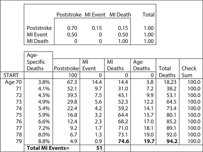
Figure 11-2. Markov model for estimating the rate of myocardial infarctions (MIs) for 70-year-old stroke survivors: Asterisk indicates assumptions for the average cohort of 100 70-year-old stroke survivors.
After the health states and cycle times have been specified and the transitions and parameters calculated, the model can be programmed.
Markov models can be solved as mathematical equations using matrix algebra, they can be programmed in spreadsheets using one column for each health state and one row for each cycle, or they can be programmed in special modeling software. Figure 11-2 shows a simple Markov model for risk of a myocardial infarction (MI) in stroke survivors. Such a model might have just three health states: poststroke, MI, and death. Thus, if we have a cohort of 100 70-year-old male patients who are discharged alive from a hospital after a stroke, and we know that the annual risk of MIs is expected to be 30% and that 50% will die from their MIs, then we can calculate the number of expected MI deaths at 10 years. However, it would be too high unless our model also accounted for competing deaths from all other causes. To correct for competing deaths, we can use actuarial life table data on the probability of death by year of age and gender (Social Security Administration, 2011). For ease of calculation, we can use spreadsheet software.
For the purpose of this illustration, we will assume that (1) the MI and death rates are constant, (2) all events happen at the end of each year, and (3) the age-specific death rates do not have to be adjusted for this stroke population. (These assumptions would be too primitive for an actual model.) This simple Markov model is depicted in Figure 11-2. The “engine” of the model is in the top box, called the “transition matrix.” In this matrix, we have translated the risks of having an MI and surviving and having an MI and dying into annual probabilities. All the row probabilities in the matrix add to 1, indicating that patients either change to a new column or stay where they are. This reflects the “mutually exclusive and jointly exhaustive” rule for Markov models. For ease of calculation, we apply the Centers for Disease Control and Prevention’s death risk first to all live patients because this death risk is age specific and increases each year. After we have estimated who dies of “old age,” then we apply the probabilities in the transition matrix to all patients on the next line of the model. Starting with 100 patients in the “poststroke” health state, at the end of the first year, we will have 14.4 patients with MIs who remain alive, 14.4 patient deaths from MI, and 3.8 deaths from old age. During the next year, we apply the same assumption to the remaining live population, and the model calculates the new numbers. In this simple example, one can see how MIs and MI deaths happen each year. You can also see how competing deaths from “old age” capture a larger and larger proportion of deaths as the population ages. If you look at the bottom of Figure 11-2, you can see that over the 10 years in the model, we had 51 MI events in which patients survived, 74.6 in which patients died, and 19.7 deaths from old age. Furthermore, the model indicates that 94.2 patients have died over the 10 years modeled. In real life, patients do not die in fractions. However, because a Markov model applies contingent probabilities repeatedly to the starting number of patients, one of its artificial features is that it will estimate fractions of people. We can circumvent this problem by calculating outcomes for large numbers of patients, or we can simply think of the Markov model results in terms of percentages of individual surviving.
SENSITIVITY ANALYSIS
Models are only as good as the assumptions and the data that are used for their construction. Decision makers, therefore, need some reassurance that predictions are not completely irrelevant to informing decisions. There are two ways to provide information about the validity of modeling results, model validation and model sensitivity analysis. Models must have face validity; that is, they must seem reasonable to experienced clinicians. If they do not, it is unlikely that they will inform any real-world clinical decisions. Models should also, at a minimum, be able to predict the prevalence of key conditions and costs for populations other than those on which they were designed (predictive validity). Unfortunately, because models are mainly needed to inform practice and policy for when strong evidence is not available, good data on outcomes for populations for the new therapies that are being modeled are often rare. If such data were readily available, then we might not need to construct a decision model in the first place. Thus, modelers must rely on examining how their estimates change as model parameters are changed. This is called sensitivity analyses. Sensitivity analyses test a model’s response to variations in the levels of parameters variables included; they answer the “what if” questions. Although parameter values are usually entered into the model as discrete values, they may be drawn from a range of potential values (i.e., confidence intervals) based on random chance or the approach to measuring. Moreover, practitioners and researchers may want to adapt the model results to slightly different populations or scenarios than those used in a model.
To test the effect of these variations on the model results, the value of a single parameter may be replaced with ones that are less likely but still possible. For example, these could include values at the limits of the parameter’s confidence interval or best or worst case scenario values. This is an example of one-way sensitivity analysis. A two-way sensitivity analysis changes the values of two parameters simultaneously. The stability of model predictions may also be tested by randomly varying many of the key parameter values within their confidence intervals. This type of testing may be done using a Monte Carlo approach.
If the model results do not change much when parameters are varied, the model is said to be stable or robust. Otherwise, the model is characterized as sensitive or volatile. One of the very important results from a modeling study is the information about which parameters most strongly affect the results. For sensitive models, we often calculate the value of the parameter at which the model yields a different conclusion; this is the model’s “tipping point.” In modeling language, this point is known as the threshold value.
SUMMARY
Comparative effectiveness research (CER) has been defined as “rigorous evaluation of the impact of different options that are available for treating a given medical condition” (CBO, 2007). Four types of research designs fall within the domain of CER: (1) systematic review or quantitative synthesis, (2) decision analysis, (3) OSs, and (4) large pragmatic clinical trials. In this chapter, we have explored how these various designs can contribute to informing treatment selection.
Large, pragmatic clinical trials offer the advantage of providing the highest quality of evidence because they randomize patients to treatment alternatives under consideration. Unfortunately, large RCTs are expensive to conduct, take comparatively long to complete, and often have restrictive inclusion criteria, making it difficult to extrapolate findings to other patient populations.
Meta-analysis or quantitative synthesis generally provides high-quality information, particularly when summarizing RCT data, but often is limited to the published literature, which may be biased toward studies with positive results. The ability to extrapolate data to populations similar to those encountered in “real–world” clinical practice also may be limited.
Models based on decision analysis are becoming more widely used because they can incorporate large and complex data that reflect routine clinical care situations. A variety of methods can be used for decision analysis purposes, ranging from relatively simple decision trees to complex Markov models. Fundamental to interpreting the results of a decision analysis is affirming both that (1) the structure of the model is valid and (2) that the data used in the model are free from bias or other errors.
Observational data may be limited by potential sources of bias related to the absence of randomization of treatment assignment. However, data from these studies may represent the typical clinical practice setting more appropriately than the constrained parameters of a clinical trial. Observational data also are available on a wide range of topics from routinely collected data and therefore may be much less expensive and time consuming for the investigator to amass.
Observational data sources include clinical record systems, as well as administrative data used for billing and regulatory purposes. These data sources often include very large patient populations that are followed over time. The lack of randomization, however, raises the question of whether the treatment groups being compared are balanced with respect to both known and unknown prognostic factors. A variety of methods have been developed to “pseudo-randomize” the study subjects, that is, to mathematically eliminate any potential bias in underlying differences between the groups being compared.
In this chapter, we have illustrated the use of a simple decision tree to evaluate a treatment guideline for managing appendicitis in children. The guideline attempts to reduce the number of children exposed to diagnostic radiation through the use of ultrasonography. The decision analysis affirmed that application of the treatment guideline dramatically lowers the use of ionizing radiation and cost. At the same time, the treatment guideline results in a slight increase in “missed diagnoses,” with a greater number of resulting peritoneal infections.
We also applied a simple Markov model to gain insight into the risk of MI incidence and mortality after a stroke. The model helps to provide an appreciation of the relative contribution of cardiac disease to poststroke mortality over time, with more nonfatal MIs in the early years, more fatal MIs and other causes in the later years, and MIs accounting for more than three of four total deaths in this group.
Comparative effectiveness research is becoming an increasingly important approach for the evaluation of treatment options and making optimal care decisions. The ability to interpret the results of CER will emerge as a crucial skill for clinicians, regardless of care setting and focus of practice.

1. Which of the following is NOT an example of comparative effectiveness research?
A. An observational study using propensity matching
B. A meta-analysis
C. An efficacy-based randomized control trial
D. A decision tree–based analytical study
2. What is one of the weaknesses related to meta-analyses?
A. They combine information from across multiple studies
B. Most of the data available will be efficacy data, not data on effectiveness
C. Similar endpoints from multiple studies are used to generate a combined effect size
D. They are not well accepted
3. Which of these is NOT a strength of observational studies?
A. Their longitudinal nature or ability for researchers to follow patients over very long periods of time that are most often contiguous
B. Their ready availability at little expense
C. Their ability to control for selection bias with randomization of subjects
D. Their ability to answer research questions that cannot be answered with RCTs such as effects of changes in policy or clinical practice
4. A stochastic decision analysis model is
A. A statistical approaches used to analyzed data to identify patterns of relationships between variables and to test hypotheses.
B. Mathematical structures that are used to link evidence from multiple sources to predict outcomes such as effectiveness, costs, or cost effectiveness often over a long time period.
C. A method used to control selection bias.
D. A way to assess the efficacy of treatment effect in clinical trials.
5. Which of these is NOT a type of propensity score method?
A. Matching
B. Stratification
C. Weighting
D. Randomization
6. What is selection bias?
A. A systematic error that can affect the integrity of a study (internal validity), causing some members of the population to be less likely to be included than others in the study sample
B. A bias that makes the results of a study difficult to generalize to a broader population
C. Error caused by study personnel being aware of the treatment allocation
D. Problems that occur related to the inability of study participants to accurately remember personal details
7. Which of these is NOT a type of data that can be used in observational studies?
A. Administrative billing data
B. Abstracted medical records
C. Survey data
D. Clinical trial data
8. The process of examining how decision analysis model estimates change as model parameters are changed is called
A. regression analysis.
B. sensitivity analysis.
C. guessing.
D. survival analysis.
9. What is NOT a benefit of large pragmatic clinical trials?
A. Maximize external validity
B. Maximize internal validity
C. Randomization controls for selection bias
D. Less expensive
10. Which of these is NOT a weakness of observational studies?
A. May lack representation of certain population groups
B. Do not contain data on patient centered outcomes such as quality of life
C. May take many years and be very expensive to obtain data
D. Diagnosis codes may not differentiate things such comorbidity, complication, or clinical severity
Stay updated, free articles. Join our Telegram channel

Full access? Get Clinical Tree


