Figure 8-1. Schematic diagram of a cohort study of the relationship between low social integration (unexposed) and risk of suicide. The shaded areas represent the unexposed persons (those with low levels of social integration).

 Example: The design of a cohort study is well illustrated by an investigation of social integration and risk of suicide conducted by Tsai and colleagues (2014). This research began in 1986 as the Health Professionals Follow-up Study (HPFS). In brief, men age 40 to 75 years who were dentists, optometrists, osteopathic physicians, pharmacists, podiatrists, or veterinarians were eligible for participation and enrolled if they completed a baseline questionnaire. The subjects were followed every 2 years with updated questionnaires. The first follow-up questionnaire in 1988 included questions on social interactions, so that became the baseline for exposure classification and follow-up. Answers to seven questions allowed the researchers to classify subjects into four levels of social integration. These questions related to marital status, size of the subject’s social network, frequency of interaction with social contacts, and participation in religious or other social groups. The responses to these questions created a summary score ranging from 1 to 12, which was then used to divide subjects into four ordinal categories of social integration. Of the 34,901 subjects who completed the social integration questions in 1988, 2937 (8%) were classified into the lowest level and 14,476 (41%) were classified into the highest level, with the remainder falling into the two intermediate categories. Subjects were followed through February 1, 2012, to determine their outcome, with particular focus on suicides.

 The HPFS large cohort study was designed as an all-male complement to the all-female Nurses’ Health Study (NHS). The widely cited NHS, now in its third iteration, has greatly advanced knowledge about a number of risk factors for leading chronic diseases. Originally designed in 1976, the primary goal was to assess the health impact of oral contraceptive use. Nurses were targeted for enrollment because it was anticipated that they would be motivated to participate in health research and had the technical knowledge to accurately report medication and other exposures.

 The first NHS enrolled more than 120,000 nurses from 11 states who were between the ages of 30 and 55 years old. After completing a baseline questionnaire, subjects were followed with repeat questionnaires every 2 years. A second NHS was launched in 1989, this time enrolling slightly younger women, age 25 through 42 years, and again resulting in a baseline study population of nearly 120,000 women. The questionnaires focused again on oral contraceptive use but also on a variety of other lifestyle factors, including diet.

 The many analyses from the NHS have produced a host of important findings. Current oral contraceptive use, for example, was linked to risk of breast cancer and cardiovascular disease but was associated with a reduced risk of colon cancer. Postmenopausal hormone use was associated with lower risk of colon cancer and hip fracture but was also associated with an increased risk of stroke and with prolonged exposure, breast cancer. Dietary analyses revealed that a Mediterranean-type diet reduced the risk of heart disease and stroke. High levels of red meat consumption were linked to both premenopausal breast and colon cancer risk. Intakes of folate, vitamin B₆, calcium, and vitamin D were all seen to lower the risk of colon cancer. These are just a sample of the findings related to this long-standing research effort.

TIMING OF MEASUREMENTS

Typically, a cohort study is prospective, meaning that the study is launched, and then exposure status is assessed in subjects followed by subsequent development of disease. All of the events of interest occur after the study begins. In the previously cited HPFS, for instance, the study was launched in 1986, exposure was defined by questionnaire responses in 1988, and subjects were followed to determine their suicide risk until 2012. Other names for this type of research design are longitudinal or follow-up studies because the events of interest are measured across time.

 An alternative approach is the so-called retrospective (or historical) cohort study in which all of the events under investigation have occurred before the onset of the study. In this version of the cohort study, one typically accesses historical records to determine exposure status and disease outcome. Here, for example, the investigator might launch the study in 2012, going back to archived records in 1988 to define exposure (e.g., social integration), and then follow death records up to 2012 to determine health outcomes.

 The rationale for conducting a retrospective cohort study may not be immediately obvious. If one considers the challenges in studying a disease that requires many years from exposure to development, however, the advantages become more apparent. For a slowly developing disease, such as cancer or heart disease, a prospective study might require decades to complete, with the answer to the research question remaining uncertain until the study could be concluded. It would be much quicker to simply avail oneself of historical information and avoid having to wait years for outcomes to occur or not. Moreover, for exposures that no longer occur, it would not be possible to conduct a prospective cohort study, and one is limited to the retrospective approach.

 The principal advantages of the retrospective cohort study design are that it provides more rapid results and that it is generally less expensive because it relies on information that is already available. The downsides of a retrospective cohort study are that historical information, whether from archived records or personal recall, may be incomplete, inaccurate, or both. Moreover, a retrospective cohort study would not be useful for evaluating a new or emerging exposure.

 Regardless of whether it is conducted in a prospective or a retrospective fashion, a cohort study often requires a large sample size, especially if the outcome of interest is uncommon. This point is well illustrated by the HPFS cited earlier in which the evaluation of social integration and suicide risk involved nearly 35,000 persons. Even with a sample size that large and nearly a quarter of a century of follow-up, only 147 suicides were observed in this study.

 The size of such a study creates many logistical challenges and can be quite expensive to conduct even if efficient methods are used to collect data, such as self-administered questionnaires and linkage to existing record sources. Attempting to follow subjects over several decades has its own logistical challenges. Individuals may move, change their names (a particular issue when following adult women, who may change their names upon marriage or divorce), elect to discontinue participation, or die from some other cause. To the extent that people who have incomplete follow-up differ from those who are successfully followed, the results of the study could be distorted. Another challenge can arise if exposure status changes during the course of the follow-up. This phenomenon was observed in the HPFS, in which 27% of the subjects traced through 8 years had decreased their level of social integration, while another 18% had increased their level of social integration. With nearly half of the subjects changing their exposure status after entry, it was important for the investigators to account for both the initial and changed exposure status in their analysis.

SELECTION OF SUBJECTS

In some situations, such as the HPFS, the subjects for a cohort study are sampled without regard to exposure status. In the HPFS, subjects had to be (1) male, (2) between the ages of 40 and 75 years old at study onset, (3) resident in the United States, and (4) a member of one of six specified health professions. In addition, subjects had to agree to participate and complete the requisite data collection instruments. A typical exclusion from a cohort study would be anyone with the outcome of interest, which in this example would not be an issue because the outcome was suicide. In other situations when the outcome of interest is not a fatal event, it would be important to exclude affected individuals. Failure to do so might distort the results or lead to mistaken inferences about the temporal sequence between exposure and disease development.

EXPOSURE STATUS

When the exposure of interest is relatively common, a general population group, such as health professionals, may be selected. In other situations, the exposure of interest may be less frequent, necessitating a strategy to enrich the study sample with exposed persons. For example, if one is interested in a study of prior suicide attempts as a risk factor for subsequent completed suicide, a general population sample likely has too few exposed individuals (prior suicide attempters). Under such circumstances, one might want to access emergency departments and mental health facilities to identify the suicide attempters to enroll in the study.

 Because the subjects in a cohort study likely will have to be followed for some time, the investigator would be well served in identifying persons who are motivated to participate and are unlikely to withdraw subsequently. The example of studying prior suicide attempters illustrates the challenges that an investigator might face in following subjects because these individuals may not be motivated to participate and may have predisposing mental health issues, social instability, and other characteristics that make them difficult to enroll and follow.

 For some exposures, it may be sufficient or necessary to classify subjects into just two levels of exposure (exposed vs. not exposed). For instance, either someone has previously attempted suicide or has not. For other situations, such as the social integration HPFS study, the exposure has multiple levels. Social integration was measured on an ordinal scale with four levels from lowest to highest. An advantage of the multiple level exposure classification is that it allows a determination of whether any association with the outcome varies in a graded fashion. Such a dose-response relationship can be useful in making inferences about whether an association is likely to be one of cause and effect. The presence of a dose-response gradient is a feature that supports a causal inference.

 The accuracy and reliability of information on exposure also is critical to reaching a valid conclusion from a cohort study. In some instances, the exposure may be assessed by a biologic marker, such as blood levels of serotonin or its metabolites in relation to suicide risk. Such measures have the advantage of being objective, and their reproducibility can be assessed readily. Unfortunately, biologic measures of exposure are not always available, such as in the case of social integration. In these situations, the investigator may have to rely on information recorded in other sources (e.g., hospital records), or as in the case of the HPFS, on information self-reported by the subjects. The latter sources of information have the advantage of ease of collection but may suffer from limitations in their quality. For example, hospital records may be characterized by incomplete information and inconsistencies in how data are classified and recorded. Self-reports may be distorted by personal perceptions and respondents’ beliefs about preferred responses. For example, in self-reports about social integration, respondents may view social isolation as an undesirable circumstance and therefore consciously or unconsciously tend to overestimate their level of social interaction. The impact of this type of misclassification may be difficult to predict, but if it occurs nondifferentially, that is, uniformly without regard to eventual outcome, it will tend to blur distinctions between or among exposure groups and thereby diminish any apparent exposure-disease association.

 Regardless of the source of information on exposure, it is desirable to demonstrate that it is reliable. That is, repeated measures on an individual subject tend to provide similar results. It is also desirable to demonstrate that the measure is accurate. That is, that it produces a classification that correctly identifies the true exposure status of individuals. Often, reliability is assessed by a substudy that examines the consistency of repeated measurements among individuals. Similarly, accuracy typically is assessed either within the study or outside of it by comparing the classification obtained with the method of interest used versus some more definitive “gold standard.”

OUTCOME STATUS

As indicated earlier, at the outset of a cohort study, it is important to ensure that none of the subjects have the outcome of interest. For a study in which the outcome is suicide, simply enrolling living subjects would avoid this problem, although one might consider additionally excluding subjects who have a history of a precursor condition, such as attempted suicide. For an outcome that is slow in developing and may have a long presymptomatic phase, such as coronary heart disease or cancer, it may be more difficult to exclude affected individuals who have undiagnosed disease. For this reason, a strategy that occasionally is deployed is to exclude from consideration any affected persons who are diagnosed within the first few years after enrollment.

 To reach valid conclusions, it is important that the level and methods of surveillance for the outcomes are comparable between exposed and nonexposed subjects. This point is well illustrated in the HPFS, in which all subjects received the same follow-up questionnaire every 2 years, there were uniform numbers of attempts (seven) to solicit responses from non-responders, and record linkage to external death information was deployed to determine outcomes for all subjects.

 An important issue is the duration of time for which subjects should be followed. The appropriate duration of follow-up is driven by several factors, including most important, the time course from exposure to disease occurrence, as well as the size of the study population and the frequency of the outcome. In terms of the time period from exposure to outcome, this can range from a matter of days for infectious diseases to decades for chronic illnesses such as cancer and heart disease. Beyond the considerations of disease time course, study duration is affected by the pragmatic concerns of having a sufficient number of outcomes to identify differences between exposed and nonexposed persons. Everything else being equal, a smaller sample size may require a longer observation period to accrue sufficient outcomes. Similarly, a less frequent outcome may require more observation time to accrue an adequate number of outcomes.

 The duration of follow-up (24 years) in the HPFS illustrates these issues well. Even though the study was quite large (nearly 35,000 subjects), the outcome (suicide) was quite rare (with 147 events in total). A shorter duration of follow-up would have resulted in proportionately fewer outcomes and may have made it more difficult to detect an effect of social integration on suicide risk.

 Information about the outcome of interest may derive from a variety of sources, including direct observation by the investigators; self-report from the subjects; or access to other record sources, such as hospital or workplace data, or as in the HPFS, from death registration information. The accuracy of cause of death information on death certificates has been questioned by multiple studies, which have found error rates exceeding one quarter of all deaths. For suicide, in particular, there may be challenges in distinguishing whether the cause of death was intentional or accidental, and if intentional, whether homicide could be ruled out. The physician, coroner, or medical examiner who certifies a death as suicide often must rely on ancillary information, such as knowledge of prior attempts, finding a note specifying intent, awareness of the presence of mental illness, and other circumstantial evidence. There also may be a hesitancy to classify a death as a suicide because of social stigmatization or legal or financial reasons. To the extent that errors are made in classifying suicides, it is likely that these events are underreported rather than overreported. As long as such errors are not differential according to social integration status, the impact on the exposure–disease association should be to blur distinctions and make it more difficult to identify a link. That is, the true low social integration–suicide association should be as strong or stronger than that observed if outcomes are misclassified nondifferentially.

ANALYSIS

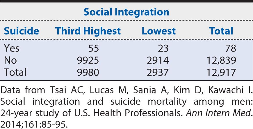
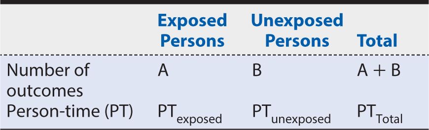
One approach to analysis of a cohort study is illustrated in Table 8-1. This format involves a simple binary classification of exposure (yes vs. no) and outcome (yes vs. no). More complicated data arrays can be constructed for multiple levels of exposure or outcome, but the basic principles of analysis are readily apparent in this basic format.

Table 8-1. Summary presentation of risk data from a cohort study.

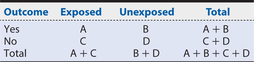
 There are four possible combinations of exposure and outcome status, as represented in the table:

   A: Exposed persons who develop the outcome

   B: Unexposed persons who develop the outcome

   C: Exposed persons who do not develop the outcome

   D: Unexposed persons who do not develop the outcome

 The risk (or cumulative incidence) of developing the outcome among the exposed persons is given by:

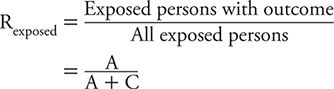
 As a reminder, risk requires a specific timeframe as a reference, such as 1 year, 10 year, and so on. Also, risk can vary between 0 (A = 0, no exposed persons develop the outcome) and 1 (C = 0, all exposed persons develop the disease of interest).

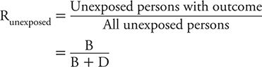
 We can calculate the risk among unexposed persons in the same manner:

Risk Ratio

We can contrast the risk among exposed and unexposed persons by dividing the former by the latter. This measure is referred to as the risk ratio (RR) and can be calculated as:

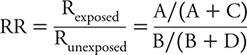
 A critical value of the RR is 1, where the risk of the outcome is identical for exposed and unexposed persons. That is, exposure has no effect on the likelihood of the outcome, or equivalently expressed, there is no association between exposure and outcome. Values of the RR above 1 correspond to situations in which the risk among exposed persons exceeds that among unexposed persons. In other words, exposure appears to increase risk or hazard to those involved. The reverse is true for situations in which the RR has a value less than 1. Here, risk among exposed persons is less than that among unexposed persons. This is equivalent to saying that exposure appears to lower risk and therefore is protective for those involved.

 The calculation of RR can be illustrated from the HPFS study of suicide. A summary of the study results is shown in Table 8-2. The risk among exposed (defined here as the highest level of social integration) is:

Table 8-2. Summary of results from Health Professionals Follow-up Study showing the suicide risk among men with the highest level of social integration compared with the corresponding risk among men with the lowest levels of social integration.

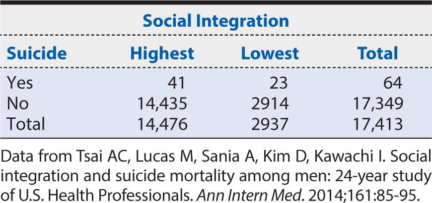
 That is, the 24-year risk of suicide among middle-aged men in the health professions with the highest social integration was about almost one third of 1%. The corresponding risk among unexposed (defined here as the lowest level of social integration) is:

 In other words, the 24-year risk of suicide among middle-aged men in the health professions with the lowest social integration was slightly more than three quarters of 1%. The RR, therefore, is calculated as:

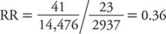
 In other words, in this population of middle-aged men in the health professions, those with the highest level of social integration had about one third the 24-year risk of suicide than those with the lowest levels of social integration. Increasing social integration, therefore, appears to be protective against risk of suicide in this population. The magnitude of this association is assessed by how far the observed RR is away from the null value of one (no association). An RR of 0.36 is consistent with a moderate to strong protective effect.

 To characterize the statistical precision of this estimate, we can calculate approximate 95% confidence intervals (CIs) around it. If we perform that calculation, the interval ranges from 0.26 to 0.50. That is, at the 95% level of confidence, the range of RR values consistent with the data observed falls between 0.26 and 0.50. The HPFS data are compatible, therefore, with an effect of high social integration on suicide risk that ranges from one quarter to half of the corresponding risk among those with the lowest level of social integration. It is worth noting that the null value of the RR (=1) is excluded from the range of values in this 95% CI. This is equivalent to stating that the association is statistically significant (at the 5% level or P <0.05). We can conclude, therefore, that an association as strong or stronger than the one observed in a sample of this size would be unlikely to arise from chance alone.

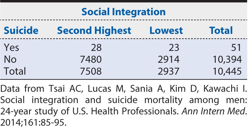
 As indicated earlier, for exposures that can be categorized in multiple ordered categories, it is possible to evaluate dose-response gradients of effect. In the HPFS of suicide, the social integration measure actually had four ordered categories. To this point, we have considered only the most extreme contrast of risk among the highest level of social integration compared at the corresponding risk for the lowest level. To examine a dose-response gradient, we can calculate an RR for each of the two intermediate levels of social integration. For purposes of consistency, we always use the same referent or baseline group as the unexposed (in this example, men with the lowest level of social integration). Table 8-3 provides a summary of the comparison of the suicide risk for the men in the second highest level of social integration compared with those in the lowest social integration category. Here, the RR is:

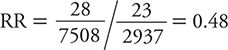
Table 8-3. Summary of results from Health Professionals Follow-up Study showing the suicide risk among men with the second highest level of social integration compared with the corresponding risk among men with the lowest levels of social integration.

 Next we calculate the suicide RR for men in the third highest level of social integration compared with those in the lowest level of social integration from the data shown in Table 8-4.

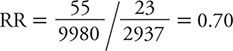
Table 8-4. Summary of results from Health Professionals Follow-up Study showing the suicide risk among men with the third highest level of social integration compared with the corresponding risk among men with the lowest levels of social integration.

 Now we have the data necessary to calculate a dose-response curve. Figure 8-2 provides a graphical summary of suicide RRs by level of social integration, with the lowest level of social integration used as the referent (RR = 1). Here we can see a progressive decline in suicide risk as social integration increases. This dose (of social integration) response (suicide risk) provides evidence to support an inference that the association is one of cause and effect.

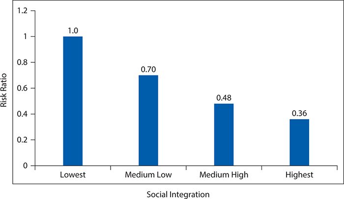
Figure 8-2. Dose-response relationship of suicide risk as a function of increasing levels of social integration among men. (Data from Tsai AC, Lucas M, Sania A, Kim D, Kawachi I. Social integration and suicide mortality among men: 24-year study of U.S. Health Professionals. Ann Intern Med. 2014;161:85-95.)

Attributable Risk Percent

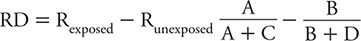
The difference in risk of the outcome of interest in relation to exposure level can be quantified in ways other than a ratio. One alternative is to subtract the risk among unexposed persons from the risk among the exposed. This measure is referred to as risk difference (RD) (sometimes also called the attributable risk). Referring to the notation introduced in Table 8-1, the RD is calculated as:

 Using the data from Table 8-2, the RD for suicide comparing the highest level of social integration to the lowest is:

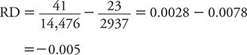
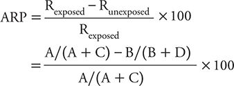
 This means that the suicide risk among men in the highest category of social interaction is 0.005 lower than that for those in the lowest category. To place this difference in risk into perspective, it is useful to scale it to the total risk (from exposure and other contributors). For exposures that increase risk, we use the total risk among the exposed as the scaling factor. This scaled measure is referred to as attributable risk percent (ARP) and is calculated as:

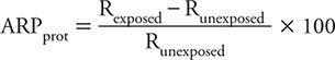
 When the exposure reduces risk, it makes more sense to scale the apparent protective effect against the total risk among the unprotected (or unexposed) group as:

 For the social integration–suicide example, this corresponds to:

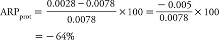
 That is to say, the highest level of social integration is associated with a reduction in the risk of suicide of 64% compared with men with the lowest level of social integration.

Rate Ratio

Thus far, we have focused on a comparison of risks, or cumulative incidence, in contrasting the experience of exposed and unexposed persons. Alternately, one can use a contrast of incidence rates (or mortality rates) for this purpose. Data for a rate comparison would appear in the format shown in Table 8-5. The rate ratio is calculated as:

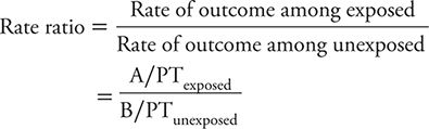
Table 8-5. Summary of incidence (or mortality) rate data from a cohort study.

where PT is person-time. As a ratio measure of comparison, the value of the rate ratio has an analogous interpretation to that of the RR. Specifically, an exposure associated with a lowered rate of the outcome has a rate ratio less than 1. An exposure that is associated with an increased rate of the outcome has a value greater than 1. When the exposure has no association with the outcome, the rate ratio is 1. The further away the rate ratio lies from 1 (the null value), the stronger the apparent association.

 The calculation of a rate ratio can be illustrated from data reported from the HPFS of suicide. In that study, the contrast of men with the highest level of social integration compared with the men with the lowest level is summarized in Table 8-6. The rate ratio is calculated as:

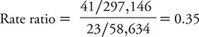
Table 8-6. Summary of results from the Health Professions Follow-up Study showing the suicide rate among men with the highest level of social integration compared with the corresponding rate among men with the lowest level of social integration.

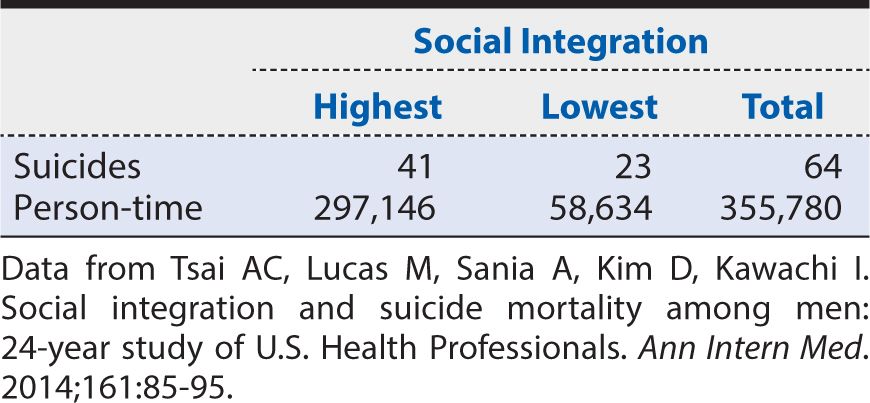
 That is, the suicide rate among men with the highest level of social integration was about one third of that for men with the lowest level of social integration. This association was unchanged by mathematical adjustment for the effect of age on the suicide rate. The investigators then went on to conduct a statistical analysis adjusting for the effects of hypertension, elevated cholesterol levels, diabetes, renal failure, employment status, smoking, alcohol use, caffeine consumption, use of antidepressants, physical activity, obesity, and having had a physical examination within 2 years. Even after all of these other characteristics were considered, the rate ratio comparing the highest to lowest levels of social integration remained 0.41. The 95% CI ranged from 0.24 to 0.69. The investigators could conclude, therefore, that increasing social integration had a moderately strong association with a lower suicide rate among men and that this association was not attributable to a large number of other characteristics, nor was it likely to have arisen by chance alone.

 The analysis of cohort studies, while following the basic principles outlined above, often involves more sophisticated statistical modeling techniques. These methods allow the treatment of the exposure (as well as the outcome) in multiple categories or as a continuous variable. In addition, mathematical models can account for the potential influence of other prognostic factors that are measured. When there are multiple variables that could affect the outcome of interest and may be differentially distributed between exposed and unexposed persons, it is important to ensure that the effects of these other variables are considered in the analysis. The approach to mathematical modeling is beyond the scope of the present discussion. For those interested in conducting analyses of cohort studies, Epi Info, a free, easy-to-use software package developed by the Centers for Disease Control and Prevention, is available at wwwn.cdc.gov/epiinfo.

SUMMARY

In this chapter, we introduced the basic principles of the conduct of cohort studies, using research on levels of social integration and suicide risk to illustrate the concepts. A cohort study is an observational (as opposed to experimental) research design in which the investigator observes the natural occurrence of exposures and disease. Sampling for a cohort study is based on exposure status, and subjects are followed over time to determine their respective risk or rate of disease development. Some cohort studies are prospective in approach. That is, all events—exposure and disease occurrence—happen after the onset of the study. Other cohort studies are retrospective in design, meaning that all of the events in question—both exposure and disease occurrence—have occurred before the onset of the study. The retrospective approach may be advantageous for diseases that are slowly developing over many years or decades by allowing faster answers, generally at much lower expense. However, retrospective studies typically rely on already available data sources, which can be incomplete or inaccurate, thereby potentially affecting the validity of inferences that can be drawn.

 Cohort studies are useful for the study of rare exposures because sampling can be based on the selective inclusion of exposed persons. In contrast, for disease outcomes that are rare, the cohort study design can be inefficient because very large study populations may be required for researchers to observe a sufficient number of outcome events. Suicide is an example of a relatively infrequent event, necessitating the study of tens of thousands of subjects.

 The analysis of a cohort study is based on a comparison of disease occurrence among exposed persons in relation to that among unexposed persons. Most often, this is expressed as a ratio measure. If the contrast is based on the risk (or cumulative incidence) of disease occurrence over a specified period of time, the measure of effect is the RR (the risk of disease among exposed divided by the corresponding risk among unexposed). The null value of the RR is 1—that is, risk of disease is not affected by exposure of interest. Values of the RR between 0 and 1 reflect lowered risk associated with exposure, with further distance from the null value indicating stronger association. Conversely, values of the RR greater than 1 correspond to increased risk associated with exposure, and again, stronger relationships are indicated by greater distance from 1. Typically, 95% CIs are calculated around the point estimate of the association to demonstrate the range of values that are statistically consistent with the observed data.

 The rate ratio is an alternate summary measure of association in a cohort study and is preferred when the focus is on the rate (either incidence or mortality or both) of disease occurrence and contrasted between exposed and unexposed persons. The interpretation of the rate ratio values is analogous to that of the RR, with a null value of 1, lowered rate among exposed indicated by values less than 1, and increased rate among exposed indicated by values greater than 1. In addition, we introduced the concept of RD and ARP as alternative ways to quantify the association of exposure and disease occurrence.

 Throughout this chapter, we illustrated basic concepts with data from the HPFS, which studied social integration level and subsequent suicide risk. For this study, a large cohort of middle-aged men in the health professions was identified in 1986, and 2 years later, nearly 35,000 of them completed a self-administered survey that allowed classification into four levels of social integration. The men were followed for 24 years to determine subsequent occurrence of suicide, of which 147 were identified. The suicide RR (95% CI) comparing men with the highest level of social integration to those with the lowest level was 0.36 (0.26, 0.50). In other words, men with the highest level of social integration had only about one third the risk of subsequent suicide as did men in the lowest level of social integration. The exclusion of the null value from the CI indicated that this association was unlikely a result of chance alone. Moreover, when graded levels of increasing social integration were each assessed against the baseline lowest level, a dose-response relationship with suicide risk was observed, falling progressively from 1 to 0.70 to 0.48 to 0.36. A similar set of findings was obtained if suicide rates were contrasted with a rate ratio measure (0.35 for the most extreme contrast of social integration levels), and mathematical adjustment for a wide range of other suspected predictors of suicide risk had minimal impact on the observed association with social integration. The HPFS, therefore, provides support for the notion that social factors are influential in determining suicide risk, at least among middle-aged male health professionals.

    1. Which of the following is NOT a feature of a cohort study?

        A. Exposure is determined by randomization.

        B. Exposure level must be assessed.

        C. Subjects are followed for the development of disease.

        D. Risk ratio is a commonly used measure of effect.

        E. It can be used to study either protective or harmful exposures.

    2. A rate ratio (95% CI) calculated from a cohort study is 1.7 (0.8, 3.4). The most appropriate interpretation is

        A. the exposure is associated with a lower rate and the result is statistically significant.

        B. the exposure is associated with a lower rate, but the result is not statistically significant.

        C. the exposure is associated with increased rate, and the result is statistically significant.

        D. the exposure is associated with increased rate, but the result is not statistically significant.

        E. none of the above.

    3. Each of the following is a feature of a retrospective cohort study EXCEPT

        A. it is efficient for the study of rare exposures.

        B. information on exposures typically is accurate and complete.

        C. it is efficient for the study of slowly developing diseases.

        D. it typically can be completed more quickly than a prospective cohort study.

        E. it may rely on already collected information.

    4. Misclassification of disease status, if it is unrelated to exposure, is expected to have what impact on the results of a cohort study?

        A. Result in a reversal of the association of interest

        B. Increase the apparent strength of association

        C. Decrease the apparent strength of association

        D. Impact cannot be predicted

    5. The null value of the rate ratio is

        A. 0.

        B. 0.1.

        C. 1.

        D. 10.

        E. infinity.

    6. If initial exposure status changes during the course of a cohort study, but this is not related to disease status, the likely impact on the strength of the apparent exposure–disease association is to

        A. increase it.

        B. decrease it.

        C. not change it.

        D. not be predictable.

    7. Cohort studies are efficient for the study of the following EXCEPT

        A. diseases that are rare.

        B. diseases with short incubation periods.

        C. exposures that are rare.

        D. exposures that are common.

    8. A dose-response relationship in a cohort study helps to support the conclusion that an association is

        A. therapeutic.

        B. statistically significant.

        C. clinically significant.

        D. biologically significant.

        E. cause and effect.

    9. Compared with a retrospective cohort study, a prospective cohort study of a particular question has what advantage?

        A. Can be completed more quickly

        B. Can be used to study exposures that no longer occur

        C. Typically is less expensive

        D. Is sufficient for studying slowly developing diseases

        E. Allows more complete and accurate information on exposures

  10. To reduce any impact in a cohort study from a clinically unrecognized disease at the outset of the study, the investigator may

        A. perform autopsies on all persons with a diagnosis of the disease of interest.

        B. eliminate from analysis all disease diagnosed in the first few years of the study.

        C. review all prior medical records and laboratory reports for exposed and unexposed subjects.

        D. consult a panel of experts in the disease of interest.

        E. blind the subjects to the exposure of interest.

Stay updated, free articles. Join our Telegram channel

Join