(1)
Department of Mathematics, University of Florida, Gainesville, FL, USA
13.1 Variability of Infectivity with Time-Since-Infection
Many diseases progress quickly. Once infected, an individual goes through a short incubation period and becomes infectious. In a matter of days, this individual has either recovered or is dead. That is the case with influenza, which many have experienced. Other diseases with short span are SARS, meningitis, plague, and many of the childhood diseases. We will call such diseases quickly progressive diseases. See Table 13.1 for a more extensive list of quickly progressive diseases. In modeling such diseases, it is acceptable to ignore host vital dynamics and to assume that the infectivity of infectious individuals is constant throughout their infectious period.
Table 13.1
Slow and fast diseases
Slow diseases | Length of infection | Fast diseases | Length of infection |
|---|---|---|---|
HIV/AIDS | Lifelong | Influenza | 2–10 days |
Hepatitis C | Lifelonga | Measles | 10–12 days |
Tuberculosis | Lifelonga | Mumps | 12–25 days |
Genital herpes | Lifelong | Rubella | 3–4 weeks |
Hepatitis B | Lifelong | Chicken pox | 17–30 days |
Cervical cancer (HPV) | Lifelong | Dengue fever | 10–30 days |
Malaria | 200a days | Ebola | 3–6 weeks |
Other diseases infect their hosts for a long time, sometimes for the duration of the lifespan of the host. Examples of such diseases include HIV/AIDS, tuberculosis, and hepatitis C. These diseases necessarily include a long-term latent or chronic stage. Such diseases are called slowly progressive diseases. Table 13.1 contains a list of slowly progressive diseases. Models of slowly progressive diseases should include host demography.
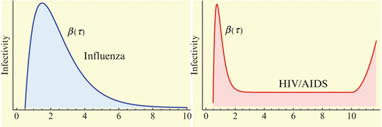
Evidence exists that the infectivity, that is, the probability of infection, given a contact, may vary in time since the moment at which the infectious individual has become infected. This variability exists with fast diseases but is far more important with slow diseases. Infectivity for several common diseases is plotted in Fig. 13.1. The problem of variability of infectivity with time-since-infection has been studied most extensively in HIV. The California Partners’ Study examined 212 females having regular sexual contacts with their HIV-infected male partners. Couples were followed for different durations (duration of exposure) up to 100 months. All partners were already infected before the contact began. Only about 20% of the females were eventually infected. Shiboski and Jewell [145] use the data to estimate a time-since-infection-dependent infectivity. No explicit form of the function is given. Generally, it is accepted that the viral load in HIV-infected patients is correlated with their infectivity. Since the viral load is high right after infection, and then during the time when AIDS develops, the infectivity is assumed to be higher for those two periods, and generally lower during the latent stage of the infection. Shiboski and Jewell’s functions do not possess these properties, presumably because infected individuals were already past their acute stage when they were enrolled in the study. Shiboski and Jewell’s functions first increase from 0 to 40 months after infection, and then rapidly decrease, so that they are nearly zero at 90 months after infection.
In fact, the very first epidemic model developed by Kermack and McKendrick [84] structures the infected individuals by the time-since-infection (also called age of infection). Kermack and McKendrick’s motivation for inclusion of infection-age was not only that infectivity may change with infection-age but also that the possibility of recovery or death may depend on the time elapsed since infection. In modeling with ODEs, it is implicitly assumed that the time to recovery or death is exponentially distributed. This assumption may be weakened if infection-age is incorporated into the model. Although Kermack-McKendrick’s age-since-infection model did not include birth and natural death in the population, more recent age-since-infection models of slowly progressive diseases include demography.
13.2 Time-Since-Infection Structured SIR Model
In this section, we consider a continuous version of the Kermack–McKendrick time-since-infection structured model. Because mass action incidence is used, the model can be used to describe diseases such as influenza and childhood diseases, but it is not suitable for HIV.
13.2.1 Derivation of the Time-Since-Infection Structured Model
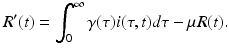
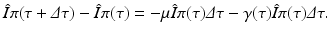
Since infectivity for infectious individuals varies with the time since infection (see Fig. 13.1), we must keep track of the time that has elapsed since infection for each infected individual. Let τ denote the time-since-infection. The time-since-infection begins when an individual becomes infected and progresses with the chronological time t. Let i(0, t) denote the number of individuals who have just become infected at time t. All individuals who become simultaneously infected make up one disease “cohort,” that is, they have experienced the same life event together, namely getting infected with the disease. As time progresses, this group of people has the same time-since-infection τ. Let i(τ, t) be the density of infected individuals with time-since-infection τ at time t. The fact that i(τ, t) is a density means that i(τ, t)Δ τ is the number of individuals with time-since-infection in the interval (τ, τ +Δ τ). Suppose that time Δ t elapses. Then the same group of individuals who at time t had time-since-infection in the interval (τ, τ +Δ τ), now at time t +Δ t have time-since infection in the interval (τ +Δ t, τ +Δ τ +Δ t). The number of those individuals is given by i(τ +Δ t, t +Δ t)Δ τ. Adding all individuals in all infection-age classes gives the total infected population:
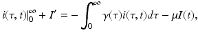
Since this is the same group of individuals, their numbers might have changed in the interval (t, t +Δ t) as a result of two possible events: some of them might have recovered, and other might have left the system due to natural causes (e.g., death). We assume that the lifespan of individuals in the system is exponentially distributed, and equal for susceptible, infected, and recovered individuals. Thus, susceptible, infected, and recovered individuals leave the system at a constant rate. Denote by μ the per capita rate at which individuals leave the system. The number of infected individuals who leave the system in the time interval (t, t +Δ t) is given by
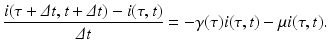
 where i(τ, t)Δ τ is the number of people in the age interval (τ, τ +Δ τ), and μ i(τ, t)Δ τ is the number of people in that age interval who leave the system at time t. To model the number of individuals who recover in the time interval (t, t +Δ t), we denote the per capita recovery rate by γ. We will assume that the recovery rate depends on the time-since-infection τ: γ(τ). Following a similar line of reasoning as in the case with the number of individuals who leave the system, the number of individuals who recover from this cohort of infecteds is given by
 The balance equation for the change in the number of infected individuals in this cohort is given by
 Dividing by Δ τ Δ t, we obtain
We rewrite the left-hand side above as
We take the limit as Δ t → 0. If the partial derivatives of the function i exist and are continuous, we can rewrite the equation above in the form
This is a first-order partial differential equation. It is linear. It is defined on the domain
 To complete the partial differential equation, we must derive a boundary condition along the boundary τ = 0 and an initial condition.
(13.1)
(13.2)
(13.3)
To derive the boundary condition, let S(t) be the number of susceptible individuals at time t, R(t) the number of recovered individuals, and N(t) the total population size:
The newly infected individuals have time-since-infection equal to zero and their number is given by i(0, t). To derive the expression for newly infected individuals, we let β(τ)N be the infectivity of the infectious individuals, where N is the total population. The infectivity depends on the time-since-infection τ that has elapsed for the infecting individual. It is assumed that infectious individuals have different infectivities at different times-since-infection. This is the case with most infectious diseases. The probability that an infectious individual with time-since-infection equal to τ will come in a contact with a susceptible individual, given that the individual makes a contact, is  . Thus, this infectious individual with time-since-infection equal to τ will transmit the disease to
 individuals. Since there are i(τ, t)Δ τ infectious individuals with time-since-infection in the interval (τ, τ +Δ τ), the total number of infections generated by such infectious individuals will be
 Adding all newly infected individuals generated by all infected individuals in all time-since-infection classes, we get
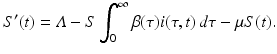
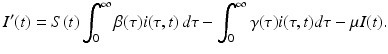
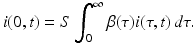 This incidence is the equivalent of mass action incidence in the ODE case. This equation gives the boundary condition of the partial differential equation. To derive the equation that gives the dynamics of the susceptible individuals, we assume that the recruitment into the population occurs at a constant rate Λ. Thus, the equation becomes
 Finally, the equation for the recovered individuals has as an inflow the total number of recovered individuals summed by all age-since-infection classes:
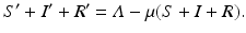
 The susceptible, infected, and recovered populations make up the total population. The equations for the susceptible, infected, and recovered populations define a closed system of equations, which we will consider in itself:
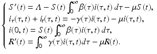
The model is equipped with the following initial conditions:
. Thus, this infectious individual with time-since-infection equal to τ will transmit the disease to(13.4)
(13.5)
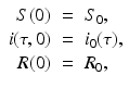
where S 0 and R 0 are given numbers, and i 0(τ) is a given function that is assumed integrable. We note that
Model (13.4) together with the initial conditions (13.5) is the time-since-infection structured Kermack–McKendrick SIR epidemic model.
Remark 13.1.
Typically, the infectivity β(τ) is assumed to be a bounded function:

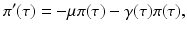
A key quantity related to the survival of infectious individuals in a given class is π(τ), the probability of still being infectious τ time units after becoming infected. Then, if  individuals become infected at some moment of time, the number of those who are still infectious after τ time units is
  . Those numbers change in a small interval of time-since-infection Δ τ by those who have stopped being infectious or those who have left the system:
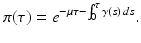
 The probability of still being infectious τ time units after becoming infected/infectious, π(τ), satisfies the following differential equation:
individuals become infected at some moment of time, the number of those who are still infectious after τ time units is . Those numbers change in a small interval of time-since-infection Δ τ by those who have stopped being infectious or those who have left the system:whose solution is
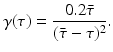
Different assumptions on γ(τ) correspond to different real-life scenarios. If all infected individuals are assumed to recover or leave the infectious class by certain age-since-infection  , their probability π(τ) of still being infectious, that is, of being in the class i, τ time units after becoming infected/infectious must tend to zero as
  . This will occur if the function γ(τ) tends to
  as
as  . Thus, we may assume that
 The corresponding probability of survival in the infectious class when μ = 0 is given by
 This probability of survival is graphed in Fig. 13.2 with
  . The coefficient 0. 2 is used to give the typical shape of the graph characterized by slow decrease for small τ and fast decrease for
  .
.
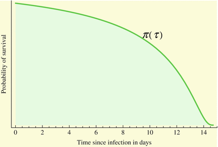
, their probability π(τ) of still being infectious, that is, of being in the class i, τ time units after becoming infected/infectious must tend to zero as . This will occur if the function γ(τ) tends to as . Thus, we may assume that. The coefficient 0. 2 is used to give the typical shape of the graph characterized by slow decrease for small τ and fast decrease for .Fig. 13.2
A typical probability of survival in a class
13.2.2 Equilibria and Reproduction Number of the Time-Since-Infection SIR Model
The model (13.4) is a first-order integrodifferential equation model. We would like to be able to say something about the solutions. Could a reproduction number  be defined such that the disease dies out if
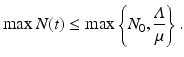
  and persists otherwise? First, one has to show that for each nonnegative and integrable initial condition (13.5), the model has a unique nonnegative solution. This result is not obvious, but the derivation is somewhat technical and will not be included. Next, we would like to see that the solutions are bounded. To see this, we must obtain the differential equation satisfied by the total population size. Integrating with respect to τ the PDE in system (13.4), we obtain
be defined such that the disease dies out if and persists otherwise? First, one has to show that for each nonnegative and integrable initial condition (13.5), the model has a unique nonnegative solution. This result is not obvious, but the derivation is somewhat technical and will not be included. Next, we would like to see that the solutions are bounded. To see this, we must obtain the differential equation satisfied by the total population size. Integrating with respect to τ the PDE in system (13.4), we obtainwhere I′ above is the derivative of the total infected population size I with respect to t. If we assume  , the above equality leads to
 Adding the equation above to the equations for S′ and R′ from (13.4), we obtain
 Thus, the total population size satisfies the usual equation, whose solution we know. In particular, we know that
, the above equality leads toNow we consider equilibria of the model. As before, to find the equilibria, we look for time-independent solutions (S, i(τ)) that satisfy the system (13.4) with the time derivatives equal to zero. The system for the equilibria takes the form
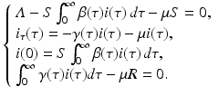
This system consists of one first-order ODE with initial condition that depends on the solution, and two algebraic equations. Clearly,  is one solution of that system. This solution gives the disease-free equilibrium, where the age-since-infection distribution of infectious individuals is identically zero. The disease-free equilibrium always exists. An endemic equilibrium will be given by a nontrivial solution
 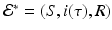 .
.
(13.6)
is one solution of that system. This solution gives the disease-free equilibrium, where the age-since-infection distribution of infectious individuals is identically zero. The disease-free equilibrium always exists. An endemic equilibrium will be given by a nontrivial solution .There is a typical approach for solving such systems. We first solve the differential equation whose solution is
This is not an explicit solution, since i(0) depends on i(τ). The following notation is useful:
 This notation occurs when we compute the total infectious population:
 The usual approach to solving the system (13.6) is to substitute the expression for i(τ) from (13.7) in the boundary condition and the total population size. We typically obtain a system for i(0) and S. However, in this case, when we substitute i(τ) in the boundary condition, we obtain an explicit expression for the susceptible individuals in the endemic equilibrium:
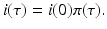
From the third equation in (13.6), we can express R in terms of i(0):
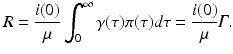
We note that Γ is a given number. To find i(0), we use the first equation in (13.6), which becomes
 Substituting S, we obtain
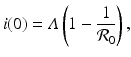
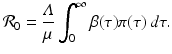
where we have defined the basic reproduction number as
 From the above expressions, we see that the endemic equilibrium is unique and exists if and only if
 ![$$ \mathcal{R}_{0} > 1 $$
” src=”/wp-content/uploads/2016/11/A304573_1_En_13_Chapter_IEq15.gif”></SPAN>.</DIV><br />
<DIV id=FPar2 class=]()
(13.7)
(13.8)
(13.9)
(13.10)
Remark 13.2.
We notice that integration by parts gives the following identity:
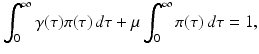 which makes each term on the left-hand side less than one. The equation above says that the probability of leaving the infectious class i through leaving the system (dying),
  , or through recovery,
 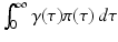 , is equal to 1. Indeed, all individuals leave the infectious class through one of those two routes.
, or through recovery, , is equal to 1. Indeed, all individuals leave the infectious class through one of those two routes.13.2.3 Local Stability of Equilibria
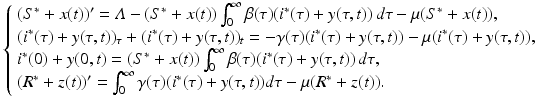
To investigate the local stability of the equilibria, we need to linearize the system. For a PDE model, that is done directly following the underlying linearization procedure. In particular, let S(t) = S ∗ + x(t), i(τ, t) = i ∗(τ) + y(τ, t) and R(t) = R ∗ + z(t), where x(t), y(τ, t), and z(t) are the perturbations, and (S ∗, i ∗(τ), R ∗) denotes a generic equilibrium. We substitute the expressions for S, i(τ, t), and R in the system (13.4):
(13.11)
Multiplying out the expressions, we have
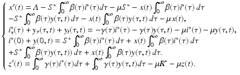
This system can be simplified further by the use of two techniques. First, we use the equations for the equilibria (13.6). This approach simplifies the system to
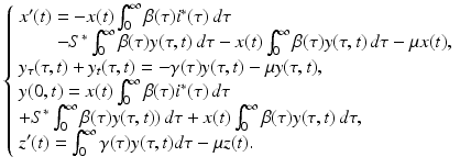
Notice that after this transformation, system (13.13) contains only terms that include a perturbation. However, system (13.13) is not linear. Terms such as  are quadratic in the perturbations. Since we assume that the perturbations are small, the quadratic terms must be much smaller. Therefore, the second technique that we use to simplify the system is to neglect the quadratic terms. After disregarding the quadratic terms, we obtain the following linear system in the perturbations:

System (13.14) is a linear system for x(t), y(τ, t), and z(t). Just like linear systems of ODEs, the above system also has exponential solutions. Therefore, it is sensible to look for solutions of the form  ,
,  ,
,  , where
  ,
,  ,
,  , and λ have to be determined in such a way that
  ,
,  ,
,  are not all zero. Substituting the constitutive form of the solutions in the system (13.14), we obtain the following problem for
  ,
,  ,
,  , and λ (the bars have been omitted):
(13.12)
(13.13)
are quadratic in the perturbations. Since we assume that the perturbations are small, the quadratic terms must be much smaller. Therefore, the second technique that we use to simplify the system is to neglect the quadratic terms. After disregarding the quadratic terms, we obtain the following linear system in the perturbations:(13.14)
, , , where , , , and λ have to be determined in such a way that , , are not all zero. Substituting the constitutive form of the solutions in the system (13.14), we obtain the following problem for , , , and λ (the bars have been omitted):(13.15)
Remark 13.3.
Solutions of system (13.15) give the eigenvectors and eigenvalues λ of the differential operator. Eigenvalues are the only points in the spectrum of operators generated by ODEs. However, operators that originate from PDEs may have other points in the spectrum besides eigenvalues, which also contribute to the stability or instability of an equilibrium. It can be shown [112] that for the problems of type (13.4), knowing the distribution of the eigenvalues is sufficient to determine the stability of a given equilibrium. In other words, we have the same rules that are used in ODEs. In particular, if all eigenvalues have negative real parts, the corresponding equilibrium is locally stable; if there is an eigenvalue with a positive real part, then the equilibrium is unstable. Because of that, we will concentrate on investigating eigenvalues.
Stay updated, free articles. Join our Telegram channel

Full access? Get Clinical Tree


