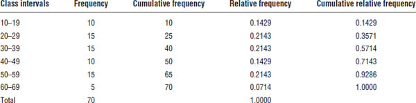
Table 9-1. A Frequency Distribution of the Ages of 100 Individuals

Measures of Dispersion

Measures of dispersion reflect variability in a set of values.

The range

One way to measure dispersion is to use the range, which is the difference between the largest value and the smallest value in the data.

Variance

The variance measures the scatter of the observations about their mean. When computing the variance of a sample, one subtracts the mean from each observation in the set, squares the differences obtained, sums all squared differences, and divides the total by the number of values in the set minus 1. The calculation of the variance of a sample can be given by

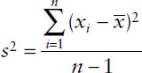
where s² stands for the sample variance, Σ is the summation sign, and stands for the sum of all values of a variable. In addition, x_i represents the ith observation for the variable X, and stands for the sample mean.

The denominator here is n − 1 because of the theoretical consideration degree of freedom. If an investigator knows n − 1 deviations of the values for a variable from its mean, the investigator will be able to determine the unknown nth deviation because the sum of deviations of all values from their mean equals zero.

The preceding equation for the calculation of variance is for sample variance. If the investigator needs to calculate population variance, the denominator of the calculation would be the total number of values in the population instead of the total number of values minus 1.

Standard deviation

The unit for variance is squared. If the investigator wishes to use the same concept as the variance but express it in the original unit, a measure called standard deviation can be used. Standard deviation equals the square root of the variance.

The coefficient of variation

The standard deviation is useful as a measure of dispersion, but its use in some situations may be misleading. For example, one may be interested in comparing the dispersion of two variables measured in different units, such as serum cholesterol level and body weight. The former may be measured in milligrams per 100 mL, and the latter may be measured in pounds. Comparing them directly may produce erroneous findings.

The coefficient of variation can be expressed as the standard deviation as a percentage of the mean, which is given by

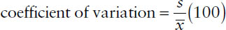
where s is the standard deviation and is the mean of the variable. Because the mean and standard deviation have the same units of measurement, the units cancel out when computing the coefficient of variation. Thus, the coefficient of variation is independent of the unit of measurement.

9-6. Evaluation of Screening Tests

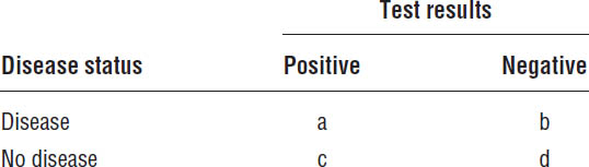
In the health sciences, investigators often need to evaluate diagnostic criteria and screening tests. Clinicians frequently need to predict the absence or presence of a disease depending on whether test results are positive or negative or whether certain symptoms are present or absent. A conclusion based on the test results and symptoms is not always correct. There can be false positives and false negatives. When an individual’s true status is negative, but the test result shows positive, the test result is false positive. When an individual’s true status is positive, but the test result shows negative, the test result is false negative. A test result can be evaluated using four measures of probability estimates: sensitivity, specificity, predictive value positive, and predictive value negative:

       ■ Sensitivity: The sensitivity of a test is the probability of the test result being positive when an individual has the disease. Using notations in Table 9-2, one can show that this probability equals .

       ■ Specificity: The specificity of a test is the probability of the test result being negative when an individual does not have the disease. Using the notations in Table 9-2, one can show that this probability equals .

       ■ Predictive value positive: The predictive value positive of a test is the probability of an individual having the disease when the test result is positive. Using the notations in Table 9-2, one can show that this probability equals .

       ■ Predictive value negative: The predictive value negative of a test is the probability of an individual not having the disease when the test result is negative. Using the notations in Table 9-2, one can show that this probability equals .

Table 9-2. Elaboration of Individuals Cross-Classified on the Basis of Disease Status and Test Results

Adapted from Daniel, 2005.

9-7. Estimation

In the field of health sciences, although many populations are finite, including every observation from the population, the sample is still prohibitive. Therefore, an investigator needs to estimate population parameters, such as the population mean and the population proportion, on the basis of data in the sample. For each parameter of interest, the investigator can compute two estimates: a point estimate and an interval estimate. A point estimate is a single value estimated to represent the corresponding population parameter. For example, the sample mean is a point estimate of the population mean. An interval estimate is a range of values defined by two numerical values. With a certain degree of confidence, the investigator thinks that the range of values includes the parameter of interest. The composition of a confidence interval can be described as

estimator ± (reliability coefficient) × (standard error)

The center of the confidence interval is the point estimate of the parameter of interest. The reliability coefficient is a value typically obtained from the standard normal distribution or t distribution. If the investigator needs to estimate a 95% confidence interval, for instance, the reliability coefficient indicates within how many standard errors lie 95% of the possible values of the population parameter. The value obtained by multiplying the reliability coefficient and the standard error is referred to as the precision of the estimate. It is also called the margin of error.

Confidence intervals can be calculated for the population mean, population proportion, difference in population means, difference in population proportions, and other measures. The first two are discussed here.

Confidence Interval for Population Mean

When estimating the confidence interval for a population mean, after calculating the sample mean, the investigator needs to determine the reliability coefficient. When the sample size is large (a rule of thumb is greater than 30), reliability coefficients can be obtained from the standard normal distribution. When an investigator needs to estimate 90%, 95%, and 99% confidence intervals, the corresponding reliability coefficients are 1.645, 1.96, and 2.58, respectively.

For example, in a study of patients’ punctuality for their appointments, a sample of 35 patients were found to be on average 17.2 minutes late for their appointments with a standard deviation of 8 minutes. The 90% confidence interval for population mean is given by

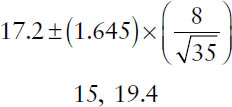
This confidence interval can be interpreted using the following practical interpretation: the investigators are 90% confident that the interval [15, 19.4] contains the population mean.

The method followed in this example applies if the sample size is large. When the sample size is small, the reliability coefficient would be obtained from a t distribution.

Confidence Interval for Population Proportion

To estimate the population proportion, an investigator first needs to draw a sample of size n from the population and compute the sample proportion, . Then the confidence interval for the population proportion can be estimated using the same composition as given for a confidence interval. When both np and n(1 – p) are greater than 5 (p is population proportion), the reliability coefficients can be estimated from the standard normal distribution. The standard error can be estimated as .

For example, among a sample of 1,000 individuals, 15% exercise at least twice a week. The 95% confidence interval for the population proportion is given by

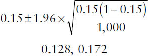
The interpretation of this confidence interval is that the investigators are 95% confident that the population proportion is in the interval between 0.128 and 0.172.

9-8. Hypothesis Testing

Both hypothesis testing and estimation examine a sample from a population with the purpose of aiding the researchers or decision makers in drawing conclusions about the population.

Basic Concepts

Null hypothesis and alternative hypothesis

When conducting research, an investigator typically has two types of hypotheses: a research hypothesis and a statistical hypothesis. A research hypothesis is the investigator’s theories or suspicions that need to be subjected to the rigors of scientific testing. A statistical hypothesis is a hypothesis stated in a way that can be tested using statistical techniques. In the process of hypothesis testing, two statistical hypotheses are used: the null hypothesis and the alternative hypothesis. The null hypothesis is the hypothesis to be tested and is typically designated as H₀. The null hypothesis is a statement presumed to be true in the study population. As the result of hypothesis testing, the null hypothesis is either not rejected or rejected. Typically, an indication of equality (=, ≥, or ≤) is included in the null hypothesis. The alternative hypothesis complements the null hypothesis. It is a statement of what may be true if the process of hypothesis testing rejects the null hypothesis. The alternative hypothesis is typically designated as H_A. Usually, the alternative hypothesis is the same as the research hypothesis.

A word of caution regarding null hypothesis is warranted here. When hypothesis testing does not reject the null hypothesis, it does not mean proof of the null hypothesis. Hypothesis testing indicates only whether the available data support or do not support the null hypothesis.

Test statistic

The test statistic is a numerical value calculated from the data in the sample. The test statistic can assume many different values, and the particular sample determines the specific value that the test statistic assumes. The test statistic can be considered as the decision rule. The value of the test statistic determines whether to reject the null hypothesis.

The general formula for the test statistic is given as follows:

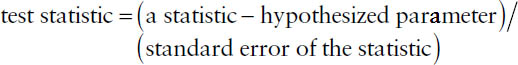
Values that the test statistic can assume are divided into two groups that fall into two regions for hypothesis testing: the rejection region and the nonrejection region. The values in the nonrejection region are more likely to occur than the values in the rejection region if the null hypothesis is true. Therefore, the decision rule of hypothesis testing is that if the value of the test statistic is within the rejection region, then the investigator should reject the null hypothesis and vice versa.

Significance level

The critical values that separate the rejection region from the nonrejection region are determined by the level of significance, which is typically designated by α. Thus, hypothesis testing is frequently called significance testing. If the test statistic falls into the rejection region, then the test is said to be significant.

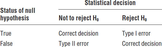
Type I and type II errors

Because significance level determines the critical values for separating the rejection and nonrejection regions of a test, an investigator obviously has a probability of committing errors when conducting hypothesis testing. There are two types of errors for hypothesis testing (Table 9-3). When the null hypothesis is true, but the statistical decision is to reject the null hypothesis, the investigator has committed a type I error. If the null hypothesis is not true, and the statistical decision is not to reject the null hypothesis, then the investigator has committed a type II error. The probability of a type I error is the level of the significance for the test, which is α. The probability of a type II error is typically designated as β. Another concept often used in statistics is power, which is the probability of not rejecting a false null hypothesis.

In a hypothesis testing, the level of significance, or α, is typically made small so that there is a small probability of rejecting a true null hypothesis. Typical levels of significance for statistical tests are 0.01, 0.05, and 0.1. However, the investigator exercises less control over the probability of a type II error. Keep in mind that the investigator never knows the true status of the null hypothesis. Therefore, to have a lower probability of committing any errors, investigators take more comfort when a null hypothesis is rejected.

The p value

The p value for hypothesis testing is the probability of seeing a test statistic that is as extreme as or more extreme than the value of the test statistic observed. Reporting p value as part of the results is more informative than reporting only the statistic decision of rejecting or not rejecting the null hypothesis.

One-sided and two-sided tests

When the rejection region includes two tails of the distribution of the test statistic in testing a hypothesis, it is a two-sided test. If the rejection region includes only one tail of the distribution, then it is a one-sided test. In other words, if both sufficiently large and small values of a test statistic lead to rejection of the null hypothesis, then the investigator needs a two-sided test. If only sufficiently large or small values of a test statistic can lead to rejection of the null hypothesis, then the investigator needs a one-sided test.

Hypothesis Testing for a Population Mean

When testing a hypothesis for a population mean, an investigator uses a Z statistic or a t statistic, depending on whether the sample size is large (this may remind readers of the determination of the reliability coefficient for the confidence interval). When the sample size is small, the investigator should use the t statistic, which is given by

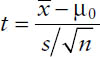
where stands for the sample mean, μ₀ represents the hypothesized population mean, s stands for sample standard deviation, and n represents sample size.

Hypothesis Testing for a Population Proportion

When one tests a hypothesis for a population proportion and when the sample size is large, the test statistic is given by

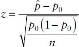
where stands for the sample proportion, p₀ represents the hypothesized population proportion, and n stands for sample size.

9-9. Simple Linear Regression and Correlation Analyses

Regression and correlation analyses are used when analyzing the relationship between two numerical variables. Regression and correlation are closely related, but they serve different purposes. Regression analysis focuses on the assessment of the nature of the relationships with an ultimate objective of predicting or estimating the value of one variable given the value of another variable. Correlation analysis is related to the strength of the relationships between two variables.

The Regression Model

Independent variable and dependent variable

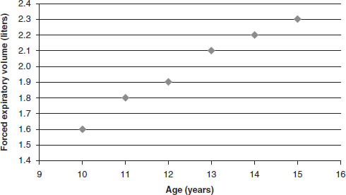
In a simple linear regression, two variables are of interest: the independent variable X and the dependent variable Y. Variable X is usually controlled by the investigator, and its values may be preselected by the investigator. Corresponding to each value of X are one or more values of Y. When the investigator conducts simple linear regression analysis, the objective is to estimate the linear relationship between the independent and dependent variables. The investigator needs to first draw a sample from the population and then plot a scatter diagram of the relationship between the two variables by assigning the values of the independent variables to the horizontal axis and the values of the dependent variable to the vertical axis. An example of such a diagram is the relationship between age and the forced expiratory volume (liters) among a group of children between 10 and 16 years of age (Figure 9-1). It is clear from this diagram that the older the children are, the greater the forced expiratory volume. In other words, a linear relationship may exist between the two variables.

Estimation of the linear line

The method usually followed to obtain the linear line is known as the method of least squares, and the line obtained is the least squares line. The least squares line has this characteristic: the squared vertical deviations of any data point from the least squares line are the smallest among all possible lines that describe the linear relationship between the independent and dependent variables.

The general format of the least squares line is 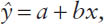where a is the sample estimate of the intercept of the line, and b is the sample estimate of the slope of the line. The population parameters for the intercept and the slope of the line are designated α and β, respectively. The estimated least squares line for the linear relationship depicted in Figure 9-1 is given by

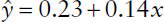
where a, the intercept of the line, has a positive sign, suggesting that the line crosses the vertical axis above the origin; and b, the slope of the line, has a value of 0.14, suggesting that when x increases by 1 unit, y increases by 0.14 unit.

Stay updated, free articles. Join our Telegram channel

Join