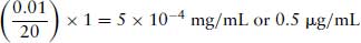
Particular care must be to ensure that all the units are the same. For example, if 10 μL of a 1 mg/mL solution is added to 20 mL organ bath, the same units must be used throughout. 10 μL is expressed as 0.01 mL. The final concentration in the organ bath is:
Frequently, it is advantageous to work in molar units throughout, starting with the stock solutions. This prevents calculation errors and it is easy to arrive at the final molar concentrations.
A few examples are given to illustrate some typical calculations.
1.5.4 Logarithms
Logarithmic relationships between variables are common in pharmacology. It is therefore important to have a clear understanding how to manipulate logarithms in calculations. When expressing numbers as logarithms, a base number must be specified. There are two commonly used base numbers, 10 (log10) and e = 2.7183 (loge, ln or natural logs). Log10 are most widely used in pharmacology. The logarithm of a number (x) is the base number (b) to the power of that number (i.e. bx). For example,
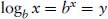
and

The term antilog is more accurately described as the exponent, or the power to which the base must be raised to equal the original number.
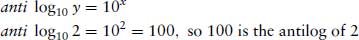
Using a calculator, the exponent or antilog is found by using the inverse log function. The order in which numbers and functions are entered varies between different models of calculator, and should be checked for each model.
Logarithms are frequently first encountered in chemistry in the pH scale which is used to express the hydrogen ion concentration. For practical purposes, pH is defined as the negative logarithm to the base 10 of the hydrogen ion concentration [H+]. Thus in a solution of pH 7, the [H+], or more accurately the hydronium ion [H3O+] is –antilog 7 = 10−7 M. Note that an increase in one unit of pH scale means that the [H+] decreases 10-fold, because

In pharmacology, a logarithmic scale is used to express the potency of a drug, be it agonist or antagonist (see Section 2.1). If an agonist has a potency (EC50) 10−6 M, then it is said to have a pD2 of –log10 10−6 = 6. In order to compare the potency of this drug with another drug with a pD2 of 8, then it may be thought that this would simply be 6/8 = 0.75, so drug A is 0.75 times less potent than drug B. This is incorrect! When the log of a number is divided by the log of another, they are in fact subtracted, and the answer is the log of the difference:
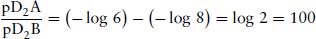
So drug A is in fact 100× less potent than drug B.
1.6 ESSENTIAL STATISTICS
This section is not intended to give a comprehensive account of statistics as applied to biomedical experiments, since this has been done in books dedicated to the topic. For a more detailed explanation of statistical procedures, recommended books are those by Ennos (2012) and Motulsky (2003). The latter refers to the explanatory manuals (available as books and online) for GraphPad Prism, and is particularly useful since the software was written by bioscientists for bioscientists, and there are regular updates and analytical tips available on their website.
From the outset, it should be clear that there are three very different types of data:
- continuous or quantitative data
- ranked data
- non-continuous or categorical data
1.6.1 Continuous Data – t-test, ANOVA, Non-parametric Tests and Regression
Continuous (or quantitative) data consist of measurements of variables such as contraction, blood pressure temperature, time or concentration. Since the basic aim of statistics is to be able to extrapolate from sample measurements of a population to the entire population, and then assess the probability that one population (treated or untreated) differs from another. To do this it is necessary to estimate the variability of sample measurements (precision), and the distribution of individual measurements. The precision is described by the variability by descriptive statistics, the mean and standard deviation. It is vital to know whether or not the sample measurements are distributed “normally”, where a bell-shaped Gaussian curve is obtained. It is simple to check the distribution of the sample measurements by simply plotting a frequency curve. It will be apparent how important it is to have a sufficient number of sample measurements. A bare minimum of 10 will start to form a pattern, but really 10 times this is needed to obtain a reliable frequency distribution curve. A table of descriptive statistics will give information about the variation of the samples in the population. This can be carried out by any statistical software package. It will consist of information about the mean and variability and confidence limits. It will convey information as to whether the distribution is symmetrical or skewed on either side of the mean. The standard deviation expresses the variation of samples around the mean, and depends how “flat” the bell-shaped curve is. If there is small variation about the mean it will reflect a sharp bell-shaped curve. The standard deviation (SD, S or σ) is defined as
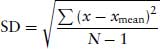
where x = each value, xmean = mean of values and N = number of values.
If the results are evenly distributed in a Gaussian manner, then 68% of the results fall within SD of the mean, and 95% of the values fall within 2SD of the mean.
The standard error of the mean (SEM)

This indicates the precision with which the true population mean has been estimated.
The appropriate statistical test to analyse quantitative data depends on the aim and design of a study. The study may have one of two basic aims.
To calculate the probability that two populations are different from each other, that is to say that they have different means (e.g. treated compared with control). The appropriate test will depend on (a) whether the measurements are “normally” distributed, and (b) the numbers of populations (e.g. treatments). Parametric tests are used to test normally distributed data, otherwise non-parametric tests must be used.
Comparing Two Populations
The method of testing for a difference between treatments is to propose a “null hypothesis”, which states that the two populations have the same mean and distribution (i.e. that they are both from a single population). Statistical tests will calculate probability that this is true or false. If it is true, the null hypothesis is accepted, and it can be said that there is a high probability that there is no difference between the populations. It is only when the null hypothesis is rejected that it can be stated that there is probability that there is a difference. The probability level commonly taken is 95%, which can be expressed as P = 0.05 or 1 in 20. This is accepted as being the minimum level of probability that is regarded as statistically significant. For normally distributed, parametric populations, a Student’s t-test can be used. To test the null hypothesis, the value of a t-statistic is calculated. This is a measure of how different the means are relative to the variability. In general, the t-statistic is calculated as the difference between the two means divided by the standard error of the difference between the means:

The t-statistic is tested against a critical value (obtained from tables or embedded in a computer program). The larger the t-statistic the greater the distance between the means, and the more likely that the null hypothesis will be rejected. The smaller the value of the t-statistic, the more likely the null hypothesis will be accepted.
For parametrically distributed populations, the t-statistic is calculated in a slightly different manner depending on the design of the experiment.
If the populations are not distributed in a Gaussian manner, a parametric test should be used. These tests compare the ranks of each sample, irrespective of the treatment group to which they belong. Examples are the Mann–Whitney test and the Wilcoxon signed-rank test.
Example of a Student’s t-test
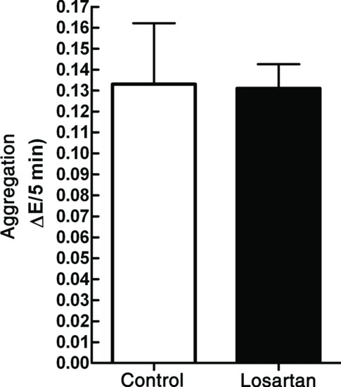
According to a report, the angiotensin receptor antagonist, losartan, inhibited platelet aggregation. This was curious because angiotensin receptors had not been reported on platelets, but if this was true it would document an additional beneficial effect of losartan, which is widely prescribed for hypertension and heart failure. A single concentration of 10 mM was used in the study. To investigate any inhibitory effect on a platelet agonist, a sub-maximal collagen concentration of 7.81 μg/mL was selected. A platelet aggregation experiment was carried out in which there were three control measurements, followed by three measurements in the presence of 10 mm losartan. A t-test was performed to statistically assess any differences between the treatments (to calculate the chances that the null hypothesis was true or false). The results obtained are shown in Table 1.1, and plotted as a bar graph in Figure 1.1.
Table 1.1 Inhibition of collagen-stimulated platelet aggregation (measured as decrease in optical density) by losartan.
| ΔE/min | |
| Control | Losartan |
| 0.155 | 0.120 |
| 0.100 | 0.130 |
| 0.144 | 0.129 |
| 0.103 | 0.151 |
| 0.136 | 0.136 |
| 0.124 | 0.129 |
| 0.115 | 0.148 |
| 0.132 | 0.144 |
| 0.102 | 0.141 |
| 0.125 | 0.137 |
Figure 1.1 Inhibition of collagen-stimulated platelet aggregation by losartan. The large bars show the means of the two samples and the error bars indicate the SEM, n = 10. A t-test is carried out to test whether there is a statistical difference between the two samples.