According to the Law of Mass Action, the value of the dissociation constant (Kd) could be derived as follows:

(2.2)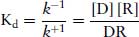

It was fully appreciated at the time that Kd is the equilibrium binding constant, and is not a functional parameter relating drug concentration to the response. If the concentration of an agonist is plotted against the response, a hyperbolic curve is found (Figure 2.1). This is analogous to the [substrate] versus velocity relationship for an enzyme reaction. Rather one of the many transforms that are used in enzyme kinetics (e.g. a Lineweaver–Burk plot introduced in 1934), agonists were characterized by their log concentration–response relationship, which was thought to validate this model (Figure 2.1).

Figure 2.1 Example of a sigmoid logarithmic concentration–response curve. Note that the potency is the concentration of the agonist required to produce 50% of the maximal response. This is the antilogarithm of the value read off the x-axis, when y = maximum response/2.

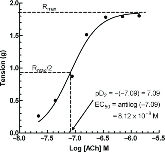
The potency of an agonist is defined as the EC50, that is, the concentration that produces 50% of the maximum response, and the pD2 is the negative log of the EC50 expressed as a molar concentration (Figure 2.1). The relative potency of two agonists A and B is EC50 of A/EC50 of B or antilog (pD2 of A – pD2 of B). The pD2 is generally less than the pKd, the reasons for which are explained shortly.

The maximum response elicited by a series of agonists acting at the same receptor frequently is not the same, although they all can occupy 100% of the receptor sites. A partial agonist is one that produces only a fraction of the maximum response compared to full agonist, even when 100% of the receptors are occupied. This fraction is referred to as the “intrinsic activity” (α). Stephenson (1956) introduced the term “efficacy” to express the ratio between response and receptor occupancy. Thus a “high-efficacy” agonist can produce its maximum response even when only a fraction of the receptors are occupied, whereas a “low-efficacy” agonist cannot produce the same maximum response even when 100% of the receptors are occupied. This situation implies that the EC50 of an agonist is not the same as the Kd as expressed in the original model proposed by Hill and Clark. An attempt to directly determine the value of Kd is made by ligand-binding experiments, which are more fully addressed in Section 9.2.3. As eloquently described by Colquhoun (2006), the term “efficacy” remained a rather elusive concept until the report of del Castillo and Katz (1957) on the action of acetylcholine acting at the nicotinic receptor ion channel at the neuromuscular end plate of the frog rectus abdominis, a type of skeletal muscle. They proposed that the receptor could exist in two states, inactive and active. The relationship between measurements of the binding of an agonist to a receptor and its response can be more usefully expressed as:

(2.3)

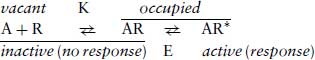
Here K is the affinity of the agonist for the receptor and E is a factor representing efficacy. The binding of an agonist to a receptor changes its conformation into a state where it can produce a response. Partial agonists can bind to form AR but do not proceed to efficiently form AR*. This is the importance of receptor coupling to signal transduction mechanisms, which are still not completely understood. There is much more insight in the case of activation of ion channels than for G-protein-mediated transduction mechanisms (Kenakin, 2006). The situation shown in Equation 2.3 is known as a binary model, where the receptor can exist in two states. Subsequently, more complex models including three or more receptor states (tertiary or quaternary models) have been proposed to account for later observations.

Another type of agonist, termed an inverse agonist, is also known. These produce a decrease in the basal response, and must be termed agonists, rather than antagonists since pure antagonists produce no response on their own. The action of inverse agonists is explained in terms of Equation 2.3 by postulating that in a resting state, in the absence of agonist, the receptor exists as an equilibrium between inactive R and active R*. An inverse agonist would then reduce the amount of receptor in the activated R* form. An example of an inverse agonist is the convulsive effects of some β-carbolines acing at the GABAA receptor. Agonists acting at this receptor, such as benzodiazepines, have sedative effects.

2.1.2 Antagonists

Antagonists act in one of the three ways:

The first category, competitive and reversible, is the most amenable to kinetic analysis and is generally the most useful therapeutically. The development of the theory of competitive antagonism ran parallel with that of competitive inhibition of enzymes (Michaelis and Menton, 1913; Haldane, 1930), yet it was not until 1959 that Schild published a practical method for experimentally determining the potency of an antagonist. Gaddum (1937) and others had approached the situation of two ligands (agonist A and antagonist B) competing for the same binding site on a receptor. When B occupies binding sites on the receptor, it will reduce the sites occupied by A. This will depend on the concentrations of A and as well as the equilibrium dissociation constants of A and B. The receptor occupancy of A was expressed by Gaddum as:

(2.4)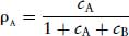

where , and , and KA and KB are the equilibrium dissociation constants for A and B, respectively.

Schild (1947, 1949, 1957) proposed a way of measuring the affinity of an antagonist for a receptor which did not depend on knowledge of the receptor occupancy, and thus avoided the obscure relationship between binding and response. Schild only considered the concentration of the agonist that is required at various antagonist concentrations to produce the same response. This made the reasonable assumption that the same receptor occupancy by the agonist will also produce the same response. Thus, in the presence of antagonist the receptor occupancy of A , when the agonist concentration is [A1]:

(2.5)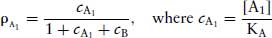

In the absence of agonist, the receptor occupancy of A with agonist concentration [A0] is:

(2.6)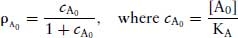

Since equal receptor occupancies of agonist produce equal responses,

(2.7)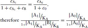

which simplifies to , where is the ratio of concentrations of agonist in the presence of antagonist and in the absence that produce the same response. This was termed by Schild as the dose or concentration ratio (CR).

So,

(2.8)

and taking logarithms,

(2.9)

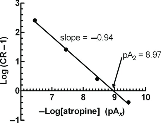
This is known as the Schild Equation. Schild was very cautious not to relate the response with the number of activated receptors, but merely assumed that equal effects involved an equal number of receptors (Arunlakshana and Schild, 1959). For this reason, he coined a term pAx = –log[B], which was defined as the negative log of the concentration of an antagonist that will reduce potency of an antagonist x times (Schild, 1949). Schild did not state that KB in the above was the equilibrium dissociation constant of the antagonist, but merely a constant (K) related to the production of the response. Schild plotted a graph of log(CR – 1) against pAx. For a competitive, reversible antagonist, a straight line will be obtained with a slope of −1. When CR = 2, then log(CR − 1) = 0 = pAx, and was termed the pA2 value, and is a measure of the potency of an antagonist (Figure 2.2). It can be confusing why it was necessary to use the pA2 scale was used rather than the well-established pKB scale. pA2 values are based on experiments where responses are measured, whereas pKB values pertain to measurements of receptor binding. Whilst these two values are usually very close, almost always the pKB is slightly greater than the pA2, and they are not interchangeable.

If a tissue is exposed to a competitive antagonist, it will cause a parallel shift of the log concentration–response curve to an agonist (Figure 2.3). The extent to which it shifts the parallel portion of the curve is measured by the CR. This is the concentration of agonist in the presence of antagonist required to produce a fixed response on the linear part of the concentration–response curve divided by the concentration of agonist required to produce the same response in the absence of antagonist.

Figure 2.2 A Schild plot of –log[antagonist, in molar units] against log (CR – 1). The pA2 value is read off the graph at the intercept of the line with x when log (CR – 1) = 0. The pA2 value does not have any units.