, xi being one reportable result as an estimate of μ. Bias—or trueness—of an assay on the other hand is the difference between the average of many reportable results (i.e. an infinite number) and μ.
Therefore one expects an assay to give results xi’s for which the relative difference (φ) from the true value (μ) of the sample is likely to be sufficiently small, for example within predefined acceptance limits λ. Stated more formally, the true probability π that a reportable result’s relative error lies within acceptance limits [-λ, +λ] should be greater than a specified quality (probability) level πmin (Hubert et al. 2004; Boulanger et al. 2007, 2010).
where Z is a standard normal random variable. Note how Eq. (16.2) relates the primary CQA π with the traditional metrics δ and σ that are discussed in ICH Q2.
(16.2)
This leads to a definition of the “acceptance region”, i.e. the set of performance parameters {δ, σ} such that the quality level π is greater than πmin. Figure 16.1 shows, below the curves, the acceptance region for various values of πmin (99, 95, 90, 80 and 66.7 %) when the λ acceptance limits are fixed at [−15 %, +15 %] as recommended for example with bioanalytical methods (FDA 2001). Logically, as can be seen from Fig. 16.1, the greater the true standard deviation σ of the assay or the greater the bias δ, the less likely a result’s relative error will fall within the acceptance limits.
Fig. 16.1
Acceptance region of analytical methods as a function of the method bias and precision when λ = 15 %
Therefore, for a given quality level πmin, all methods whose true performance criteria {δ, σ} are inside the corresponding acceptance region should be likely accepted after validation experiments, while methods with performance outside the same regions should in most case be rejected. The higher is the required quality level πmin, say 99 %, the smaller is the region representing potential assays able to fulfil this requirement.
16.3.2 Objective of Validation of an Assay
The objective of a validation or qualification phase is to collect, using proper experimental designs, information about the performance of the assay. Performance measure estimates of bias and precision permit a calculation of the probability that the assay will provide, in the future, a given result’s relative error within the acceptance limits [-λ, +λ]. The expected probability  of a future result’s relative error that will fall within the acceptance limits, given the estimated performance of the assay is:
There are several potential statistical approaches available for calculating the probability of future results from unknown samples falling within the specifications. This is further discussed in Sect. 16.4.
of a future result’s relative error that will fall within the acceptance limits, given the estimated performance of the assay is:(16.3)
16.4 Decision Rules About Primary CQA
16.4.1 Suitable Decision Rule
Good decision-making during validation implies rejecting analytical methods whose true performance (δ, σ) are not included in the acceptance region (i.e., of Fig. 16.1) while accepting analytical methods whose performance (δ, σ) are in the acceptance region, for a given quality level πmin. However, as the true bias and the precision are unknown and estimated from data, a decision rule has to be defined as a function of performance parameter estimates. Most common decision rules for analytical method validation are presented in Sects. 16.4.1 and 16.4.2.
Figure 16.2b represents a sketch of a suitable decision rule for an acceptance level πmin = 80 % and a true bias δ = 6 % as a function of true σ. The vertical line is at σ = 10 %, i.e. the top of acceptance region in Fig. 16.2a for the corresponding πmin = 80 % and bias δ = 6 %. That is, a perfect decision rule should accept all methods with  and reject all methods with
 ![$$ \sigma >10\% $$
” src=”/wp-content/uploads/2016/07/A330233_1_En_16_Chapter_IEq4.gif”></SPAN>. However, every decision rule involves risk. For this reason, the acceptance line in Fig. <SPAN class=InternalRef><A href=]() 16.2b is S-shaped rather than appearing as an ideal step function. The red shaded area represents the laboratory risk because these are methods that are truly acceptable but rejected by the decision rule, while the green shaded area represents the consumer risk because these are the methods which are truly not acceptable, but are accepted. The purpose is therefore to propose a unique decision rule that will minimize both risks, for a given, reasonable, and effective sample size.
16.2b is S-shaped rather than appearing as an ideal step function. The red shaded area represents the laboratory risk because these are methods that are truly acceptable but rejected by the decision rule, while the green shaded area represents the consumer risk because these are the methods which are truly not acceptable, but are accepted. The purpose is therefore to propose a unique decision rule that will minimize both risks, for a given, reasonable, and effective sample size.
and reject all methods with Fig. 16.2
(a, b): Example of suitable “decision rule” for an acceptance level πmin = 80 % and a true bias δ = 6 % as a function of true σ
Historically the decision about the validity of an assay was based on the estimated bias and precision. The decision was driven by frequentist hypothesis testing concepts on parameters. An assay was declared as acceptable if the estimated bias and the variance were smaller than some arbitrary limits using appropriate hypothesis testing methods and corresponding type-I error levels. Such a decision rule cannot be recommended since the primary CQA of an assay is the accuracy of its future results and not its current estimated bias and precision performance. In addition, unknown complexities are introduced by defining acceptance limits on bias and precision, when the objective is all about the quality of the results. The user of the results will make a decision about a batch, such as whether to release a batch, or about the stability of a product, based on the individual reportable results. This decision will not be based on the estimated performance of the assay that generated the results. There are several established statistical solutions to relate the estimated performances to the quality of the results. They subtly differ depending on how the assay validation rule is formulated.
Note that following decision rules are based on the assumption that the true relative error of a measurement can be obtained. That is, that the true value is known. In practice, it might not always be the case and an additional uncertainty on the reference value must be taken into account. This is beyond the scope of this chapter.
16.4.2 Risk-Based Decision Rules
The first family of solutions utilizes a risk-based formulation: what is the risk of observing future reportable results that will be unacceptably far from the true value of the unknown sample? The direct and natural option is to use the predictive distribution of future results’ relative error and to compute the predictive probability of falling within the acceptance limits. This can be obtained using Bayesian modelling and can be easily derived whatever the underlying distribution of the results and for a wide variety of experimental designs, including nested and unbalanced designs. Under the assumption of normally distributed results, non-informative priors and for a one-level nested design, the posterior predictive distribution is a t-distribution (Fig. 16.3). This distribution forms the basis of the β-expectation tolerance interval (Box and Tiao 1973; Hamada et al. 2004; Lebrun et al. 2013). Fortunately, t-distribution functions are incorporated into widely available spreadsheet packages. This avoids the need for complex numerical methods or computer programing. When working with the predictive distribution of future results’ relative error, the risk-based decision to declare an assay as valid is made when the predictive probability of falling inside the acceptance limits is greater or equal to the predefined quality level πmin.
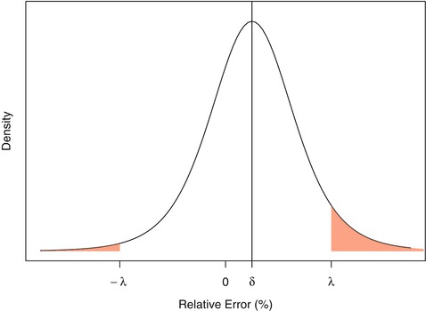
Fig. 16.3
Representation of a non-centered t-distribution. Shaded red area represents the probability that a result’s relative error will fall outside the acceptance limits
16.4.3 Interval-Based Decision Rules
The other family of solutions is based on the tolerance intervals that should be totally included within the acceptance limits for declaring an assay as valid. Again two options are possible, the first one being based on the β-expectation tolerance interval (Guttmann 1970; Mee 1984; Hubert et al. 2007a, b), which is in fact a prediction interval. The second option is to use the β-content, γ-confidence tolerance interval (Mee 1984; Hoffman and Kringle 2005), often referred to as the beta-gamma tolerance interval. This interval is commonly used in practice but not recommended for decision making in validation of assays, as it will be shown.
16.5 Predictive Distribution and Tolerance Intervals
16.5.1 Bayesian Predictive Distribution
Let’s first envisage the problem in a simple case, i.e. assuming all measurements are drawn from a unique normally distributed population having a single component of variance σ2. In that case, assuming identical, independent, normally distributed errors:
As already stated, the true performance metrics of the method (δ, σ) are unknown and must be estimated during the validation experiments.
(16.4)
The posterior distribution of the performance parameters of the method is, according to Bayes rule, proportional to the product of the likelihood [Eq. (16.1)] and the prior distribution on the parameters, i.e.:
where data refers to a set of n independent errors, φ i , obtained during validation.
(16.5)
To compare with the frequentist estimates, non-informative independent priors are assumed on the parameters. In that case, one can show that the joint posterior on the performance parameters is:
![$$ P\left(\delta, {\sigma}^2\Big| data\right) \propto {\sigma}^{\frac{2}{n}-1} \exp \left\{-\frac{1}{2\sigma}\left[\left(n-1\right){s}^2+n{\left(\overline{\phi}-\delta \right)}^2\right]\right\} $$](/wp-content/uploads/2016/07/A330233_1_En_16_Chapter_Equ6.gif)
where  is the average of all n data values, s is the usual estimate of σ, and
 ![$$ {\sigma}^{\frac{2}{n}-1} \exp \left\{-\frac{1}{2\sigma}\left[\left(n-1\right){s}^2+n{\left(\overline{\phi}-\delta \right)}^2\right]\right\} $$](/wp-content/uploads/2016/07/A330233_1_En_16_Chapter_IEq6.gif) is proportional to the likelihood function of the parameters of a normal distribution.
is proportional to the likelihood function of the parameters of a normal distribution.
(16.6)
is the average of all n data values, s is the usual estimate of σ, and is proportional to the likelihood function of the parameters of a normal distribution.Given the model and the posterior parameter distributions, the challenge in validation is to estimate the distribution of future measurement errors ϕ*? This can be addressed by computing the posterior predictive distribution of the future values of ϕ* conditionally on the available information, i.e. the data obtained during the validation experiments. Again, using Bayesian developments, one can show that the distribution of future measurement errors ϕ* is:


(16.7)
< div class='tao-gold-member'>
Only gold members can continue reading. Log In or Register to continue
Stay updated, free articles. Join our Telegram channel
Full access? Get Clinical Tree
