(1)
Department of Biology, Johns Hopkins University, Baltimore, MD, USA
Abstract
Instantaneous fluorescence emission spectra measured at different times after excitation often shift to the red as the delay between the excitation pulse and fluorescence detection is increased. In the case of Trp fluorescence in proteins, the time-dependent red shift (TDRS) may have its origins in relaxation, heterogeneity, or a mixture of the two. In those cases where it is possible to rule out the contribution of heterogeneity, the TDRS can be used to study nonequilibrium relaxation dynamics of the protein matrix and the solvent on the picosecond and nanosecond time scales. Here we describe the experimental and computational procedures involved in recording spectrally and time-resolved fluorescence, detecting heterogeneity, and extracting information about protein/solvent relaxation dynamics.
Key words
Tryptophan fluorescenceTime-correlated single-photon countingSolvent relaxationDynamic Stokes shiftTime-dependent red shiftHeterogeneous fluorescence1 Introduction
Fluorescence emission intensity from a large ensemble of fluorophores excited at time zero by a very short pulse of radiation (δ-excitation) can be described by a function of two variables: a spectral variable and the time t after excitation. Two alternative spectral variables will be used here: λ, the emission wavelength, and v, the emission wavenumber (v = 1/λ). Depending on the choice of the spectral variable, the function of two variables will be denoted either F λ (λ,t) or F v (v,t). These functions can be thought of as surfaces in 3D space, where the x coordinate is the spectral variable (λ or v), the y coordinate is the time (t), and the z coordinate is the fluorescence emission intensity. Slices of these surfaces by the planes parallel to the x and z axes represent instantaneous fluorescence emission spectra at different times after excitation. Slices of these surfaces by the planes parallel to the y and z axes resemble fluorescence decay curves measured at different emission wavelengths or wavenumbers.
The functions F λ (λ,t) and F v (v,t) contain information about the heterogeneity of the excited fluorophore ensemble and about the nonequilibrium relaxation dynamics triggered by the excitation. Theoretically, four different combinations are possible. First, we will consider the case where the ensemble is homogeneous and there is no relaxation in the excited state. In this case each of the functions F λ (λ,t) and F v (v,t) is a product of one function of the spectral variable and the other function of time, i.e.,
(1)
(2)
Here the functions f λ (λ) and f v (v) represent the spectral densities of the emitted photons on the wavelength scale and on the wavenumber scale, and τ is the lifetime of the excited state. Note that the decay curves are monoexponential and the lifetime has the same value at all emission wavelengths (or wavenumbers). If these conditions are not met, then the functions F λ (λ,t) and F v (v,t) cannot be represented in the form 1 and 2, and therefore the ensemble is heterogeneous and/or relaxation is present.
The second case to be considered involves a heterogeneous fluorophore ensemble without relaxation. For the sake of simplicity, we will assume that the heterogeneous ensemble consists of a finite number N S of homogeneous sub-ensembles, the emission of which can be described by Eqs. 1 or 2 but with different spectral distributions f λn (λ) and f vn (v) and different lifetimes τ n , where the index n = 1,2,…,N S denotes different populations. Since fluorescence emission intensities are additive, the functions F λ (λ,t) and F v (v,t) are merely the sums over all sub-ensembles:

(3)
(4)
The third case to be considered involves a homogeneous ensemble with relaxation. It has been shown [1–3] that the emission from a homogeneous ensemble of fluorophores in a relaxing host matrix can be represented in the form
![$$ {{F_{v }}\left( {v, t} \right) = {v^3}S\left[ {v -{v_{\mathrm{ c}}}(t)} \right]D(t)} $$](/wp-content/uploads/2017/03/A299540_1_En_9_Chapter_Equ00095.gif)
(5)
Here the factor v 3 takes care of the fact that under all circumstances the spontaneous emission rate is proportional to the cube of the emission frequency. The function S(x) represents the vibrational envelope of the electronic transition responsible for fluorescence emission; by definition [1, 2] this function has the following properties: ∫S(x)dx = 1, ∫xS(x)dx = 0, where the integration is carried out from −∞ to +∞. The function v c(t) represents the time variation of the spectral center of gravity of F v (v,t)/v 3,
(6)
This function describes the dynamics of the time-dependent red shift (TDRS) and contains information about the relaxation of the protein matrix and the solvent. The function D(t) represents the time variation of the product of the squared magnitude of the electronic transition dipole moment and the size of the excited-state population [1–3]. It is also known as the damping function [4–7]. If we disregard the time variation of the electronic transition dipole moment, then D(t) will also represent the decay of the excited-state population [3]. Whether the transition dipole moment is constant or varies with time, the damping function can be expressed directly in terms of F v (v,t):
(7)
The functions v c(t) and D(t) can be parametrized using linear combinations of exponential terms. It has been shown [1, 2] that such parametrization together with the expansion of the function S(x) in Taylor series makes it possible to transform Eq. 5 to the following form:
(8)
The first theoretical derivation of an expression equivalent to Eq. 8 for an ensemble of fluorophores exhibiting a time-dependent spectral shift can be found in the work of Gakamsky et al. [8, 9]. Theoretically, the number of exponential terms N E in Eq. 8 is infinite, which is a direct consequence of the infinite number of terms in the Taylor expansion of S(x). However, in the Taylor series the term becomes smaller and smaller with an increase in the term power, which makes it possible to truncate the series after just a few terms. Even if we do not neglect very small terms in the Taylor series, all but a finite number of the terms in the sum Eq. 8 will have their time constants τ n shorter than the time resolution of the experimental setup that will be used to measure spectrally and time-resolved fluorescence. This means that for all practical purposes, N E is a finite number and usually quite small (does not exceed 7).
Equations 4 and 8 are remarkably similar; if we set N S = N E and f vn (v)/τ n = α vn (v), then they become completely identical. Yet, Eq. 4 describes the emission from a heterogeneous ensemble of fluorophores without relaxation, while Eq. 8 describes the emission from a homogeneous ensemble of fluorophores in the presence of relaxation. This shows that it may be difficult to experimentally distinguish between the two cases. From the conceptual point of view, the main difference between the two cases is that in Eq. 4 N S is the number of different fluorescent species with different lifetimes τ n , whereas in Eq. 8 N E is not the number of species and τ n are not even lifetimes. Another important difference is that since the functions f vn (v) represent the steady-state emission spectra of different species, the values of f vn (v) are not allowed to be negative in any part of the emission spectrum. On the contrary, the functions α vn (v) are, generally, some linear combinations of the function v 3 S(v−v c) with its derivatives with respect to v c. The derivatives have both positive and negative values; therefore the functions α vn (v) often have negative values. Thus, the presence of negative values in some of α vn (v) can be used as the evidence that relaxation takes place in the fluorophore ensemble. Unfortunately, the absence of negative values in α vn (v) does not rule out relaxation, as well as the presence of negative values in α vn (v) does not rule out heterogeneity.
If the fluorophore ensemble is permanently heterogeneous, then the TDRS calculated in accordance with Eq. 6 contains contributions from both relaxation and heterogeneity, which are impossible to separate; this TDRS is not an accurate representation of protein and solvent relaxation dynamics. For this reason it is important to have a criterion to distinguish between a homogeneous and a heterogeneous fluorophore ensemble. One such criterion [2] uses the fact that for a homogeneous ensemble, the full width at half maximum FWHM (along the variable v) of the function F v (v,t)/v 3 does not change with time. Furthermore, when F v (v,t)/v 3 (considered as a function of v for t = const) is peak normalized, the shape of the resulting spectrum does not change as it shifts to the red (parallel translation) with increasing t. Empirically the shape conservation of the normalized spectra on the wavenumber scale during a red shift was first observed with a solvatochromic fluorescent dye 2-p-toluidinonaphthalene-6-sulfonate adsorbed to apomyoglobin or membranes [5, 6], then with indole in glycerol [1], and later with tryptophan residues in proteins [2, 3]. Theoretically, the shape conservation follows directly from Eq. 5 that was first derived in [1] under the assumption that the Franck–Condon factor envelope does not change as the spectrum shifts to the red. It must be emphasized that the width and shape conservation is characteristic of fluorophore ensembles without permanent or long-term heterogeneity. In a fluorophore ensemble where the difference between two or more sub-ensembles is conserved for the entire life of the excited state, the instantaneous emission spectrum is expected to shrink at late times, when one of the sub-ensembles outlives all the others.
This chapter describes experimental and computational procedures that are critical for obtaining the corrected (for instrumental artifacts) and smooth function F v (v,t), which is suitable for applying the shape conservation criterion and obtaining the TDRS for tryptophan residues in proteins.
2 Experimental Data Collection
Three kinds of measurements are required to generate spectrally and time-resolved fluorescence intensity surfaces F λ (λ,t) and F v (v,t) for Trp residues in proteins. First, a time-correlated single-photon counting (TCSPC) instrument equipped with monochromators and polarizers records the “decay curves” at multiple emission wavelengths. Second, a steady-state instrument with a known spectral sensitivity curve measures the steady-state emission spectrum of the same protein sample. Third, an absorption spectrum of the same protein sample is obtained using a spectrophotometer (it will be used for the inner-filter correction). The order of the measurements is important, since each of these measurements increases the concentration of photobleached Trp residues, the emission from which contaminates the fluorescence signal (see Note 1). The contamination has the most detrimental effect on the results of the time-resolved measurements, an insignificant effect on the steady-state spectra, and virtually no effect on the absorption spectra.
2.1 TCSPC Measurements
1.
Wavelengths. TCSPC decay curves are measured through a monochromator (in the fluorescence emission path) at multiple equally spaced emission wavelengths between 300 and 450 nm, at 5-nm intervals. For those proteins that also contain tyrosine residues, the optimum exciting wavelength is 296 nm; for proteins without tyrosines, it may be better to excite near 289 nm (this increases the amplitude of the TDRS). The optimum spectral resolution of the monochromator in the emission path equals 8 nm; however, for weakly fluorescent or low-concentration protein samples, it can be increased to 16 nm to effectively quadruple the sensitivity. If the excitation is at 296 nm and the protein solution scatters light too much, then the shortest emission wavelength is set to 305 nm rather than 300 nm. The decay curves are measured starting from the longest wavelength (450 nm) and ending with the shortest wavelength (300 nm), since the concentration of photobleached Trp keeps increasing during the experiment and the contamination from photobleached Trp emission has the most detrimental effect at wavelengths above 380 nm (see Note 1).
2.
Photobleaching. To avoid severe local photobleaching at the focus of the exciting beam, the beam is defocused so that its diameter is 1.5 mm at the center of the sample cell and attenuated (using neutral density filters) to 5.0 μW or less in the case of 296-nm excitation (2.0 μW or less at 289-nm excitation). The protein solution is stirred naturally every time when the protein cell is swapped with the scatterer cell (see below); therefore no magnetic stirring is needed to refresh the protein solution within the active volume. To avoid photobleaching the entire volume of the cell, the protein solution is replaced after H hours of measurements, where H = C ċV/P, C = 10 μW h/mL for 296-nm excitation, C=4 μW h/mL for 289-nm excitation, V is the volume of the protein solution in mL, and P is the mean power of the exciting beam in μW. The minimum volume of protein solution equals 1.5 mL. All measurements are performed in 10 mm by 10 mm quartz cell with all sides polished. Cells of smaller size increase photobleaching beyond acceptable levels, probably due to restricted convection in a narrow cell.
3.
Polarization. Fluorescence is excited with polarized radiation, and fluorescence emission path contains a polarizer before the monochromator. The “magic angle” configuration is used to cancel all effects of rotational diffusion on the recorded data. The “magic angle” configuration is achieved when cos2 θ exc·cos2 θ em = 1/3, where θ exc and θ em are the angles between the electric vector of the exciting and emission radiation, respectively, and the direction (usually vertical) of the normal to the plane containing the optical axes of both the exciting beam and the emission beam. For example, if the optical axes of the exciting and emission beams are horizontal and the exciting radiation is vertically polarized (θ exc = 0), then the polarizer in the emission path is set at θ em = 55°.
4.
Time resolution. The overall time resolution of the TCSPC instrument depends on the exciting pulse width, the optical pulse broadening in the monochromator, the electron transit time dispersion in the microchannel plate photomultiplier, the bandwidths and noise levels of electronic preamplifiers, and the quality of the discriminators (either constant-fraction or pico-Timing discriminators). The overall time resolution in Eq. 20can be characterized by the FWHM of the impulse response function (IRF). An IRF FWHM of 55–70 ps is desirable; 100 ps or longer is unacceptable.
5.
IRF recording. A cell of the same material and shape as the cell containing the protein solution is filled with a scatterer solution and also placed in the motorized slide (or turret) for the TCSPC measurement. The scatterer cell is used to measure the IRF quasi-simultaneously with the decay curve: out of each minute of photon counting, photons from the protein solution are counted for 50 s with the monochromator set to the emission wavelength, and photons from the scatterer solution are counted for 10 s with the monochromator set to the excitation wavelength (these are the real times rather than the live times; see Note 2). Photon counts from the protein and from the scatterer are stored in different memory segments of the multichannel analyzer (MCA), since transferring the data from the MCA to a computer takes longer than swapping the two cells and moving the monochromators between the two wavelengths (see Note 3). The mechanics of the slide or turret must have enough precision to ensure that the physical positions of different cells (when they are in the beam) differ by no more than 0.1 mm. The group velocity of light in the scatterer solution must match that in the protein sample, i.e., if the protein solvent is water, then the scatterer must be also in water; however, if the protein solvent contains 80 % glycerol, then the scatterer solution must also contain 80 % glycerol. Millimolar concentrations of ions that are commonly present in pH buffers, such as Na+ or H2PO4 −, have insignificant effect on the group velocity and do not need to be duplicated in the scatterer solution. Ludox colloidal silica is used to make water-based scatterer solutions. The concentration of Ludox is adjusted to match within 10 % the number of scattered photons per second with the number of protein fluorescence photons per second at the peak emission wavelength.
6.
Duration. The goal is to register approximately 250 millions of fluorescence emission photon counts at all emission wavelengths together. The decay curves measured near the emission maximum usually have about 16 million counts per curve; those measured at 300 nm and at 450 nm have less than one million. To avoid pileup problems, the mean rate at which emission photons are detected must not exceed 1/200 of the excitation pulse rate, which equals 4.1 MHz in our experimental setup and cannot be made much higher than that because there must be sufficient time for the excited-state population to decay completely to zero before the next excitation pulse arrives. It takes 800 s to register 16 × 106 photon counts at 20 × 103 s−1 mean counting rate; however, if the dead time and quasi-simultaneous IRF recording are taken into account, then 800 s becomes about 20 min. With 20 min per wavelength and 31 wavelengths, the duration of the entire TCSPC experiment is over 10 h. This time can be cut in half if two identical fluorescence emission wings are used in parallel (T-format) as shown in Fig. 1 (see Note 4). TCSPC data from each wing are saved in separate computer files and later combined together using the program comb_tcp, which will be described in Subheading 3.2. The program shifts the decay curves and corresponding IRF before the addition to ensure the minimum possible width of the IRF for the combined data. Whether one or two wings are used to measure fluorescence emission, if the duration of the measurement at one wavelength exceeds 300 s, then the measurement is split in two or more parts of equal duration, and the results are saved in separate files to minimize the broadening of the IRF due to slow drifts in the instrument. The data are later combined using the program comb_tcp.
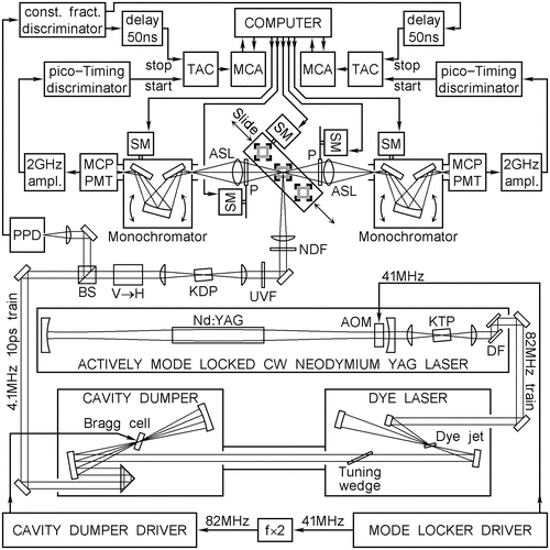
Fig. 1
Schematic diagram of the experimental setup used to collect TCSPC data. Acousto-optical modulator (AOM), aspheric lens (ASL), beam splitter (BS), dichroic filter (DF), potassium dihydrophosphate nonlinear optical crystal (KDP), potassium thallium phosphate nonlinear optical crystal (KTP), multichannel analyzer (MCA), microchannel plate photomultiplier (MCP-PMT), neutral density filter (NDF), neodymium-doped yttrium aluminum garnet (Nd:YAG), dichroic film polarizer (P), picosecond photodiode (PPD), synchronous motor (SM), time-to-amplitude converter (TAC), vertical-to-horizontal polarization rotator (V → H), ultraviolet-transmitting visible absorbing filter (UVF)
7.
Experimental setup. A schematic diagram of the experimental setup that satisfies these requirements and was actually used to collect TCSPC data in references [1–3] is shown in Fig. 1. The motorized slide carries three jacketed cell holders, two of which are hooked up to a water bath thermostat by flexible PFA tubing and can be used in the temperature range from −50 °C to +100 °C (at T < +5 °C ethanol or methanol is added to water). The third cell holder always carries the scatterer cell and works at room temperature.
8.
Calibration. Wavelength is automatically calibrated by the computer using a low-pressure Hg discharge lamp; wavelength accuracy is 0.4 nm and reproducibility 0.2 nm. Polarizers are motorized and automatically calibrated by the computer using highly polarized scattered light from a Ludox scatterer cell; calibration accuracy is 0.6° and reproducibility 0.2°. The timing calibration is achieved by manually replacing a short RG-58 cable between a pico-Timing discriminator output and the start input of a TAC by a longer cable of the same type. This introduces a calibrated delay of 19.960 ns and shifts the IRF peak to a different MCA channel. The TACs in both wings are adjusted so that the shift of the IRF peak equals 1,500 channels (see Note 5). This defines the time scale of 13.307 ps per channel. For different wings the IRF peaks can be in different channels, and for each wing the IRF peak can shift by as much as ten channels during 5 h; this is considered acceptable. The position of the peak is not as important as the time scale, which is kept constant and equal for both wings. A typical IRF is shown in Fig. 2, on the linear Y scale (top panel) and on the logarithmic Y scale (bottom panel).
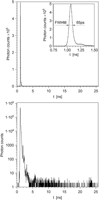
Fig. 2
Typical impulse response function (IRF) of the instrument shown in Fig. 1, plotted on the linear intensity scale (top panel) and on the logarithmic intensity scale (bottom panel). The inset in the top panel depicts the IRF on an expanded time scale and reveals its full width at half maximum (FWHM). The plot on the logarithmic scale (bottom panel) reveals several small-intensity satellite peaks resulting from the reflections of light by miscellaneous optical elements. The highest satellite peak has about 1/500 of the intensity of the main peak; on the linear intensity scale (top panel), this peak is invisible
2.2 Steady-State Emission Spectrum
1.
Wavelengths. The steady-state emission spectrum is measured using a SLM-48000S spectrofluorometer (or a comparable instrument) by scanning the emission monochromator over the wavelength range from 280 to 480 nm and recording fluorescence emission intensity at 1-nm wavelength steps. The slits of the emission monochromator are set to 4-nm spectral resolution. The slits of the excitation monochromator are set to 2-nm spectral resolution. The excitation monochromator is set to the same wavelength that was used to excite fluorescence in the TCSPC measurement, and the protein solution is thermostated at the same temperature as in the TCSPC measurement. The emission spectrum of the protein solution is recorded four times. The emission of a “blank” cell containing the same solvent without the protein is also recorded four times. The mean blank spectrum is then subtracted from the mean protein spectrum.
2.
Photobleaching. It was empirically found that in the case of the SLM-48000S spectrofluorometer, using 2-nm slits on the excitation monochromator and continuous stirring with a small magnetic stir bar is sufficient to reduce photobleaching to insignificant levels during a typical 20-min measurement. As a precaution, the spectra of the four individual scans are monitored during the measurement; a systematic decrease in the peak intensity from the first scan to the second, third, and fourth serves as a good indicator of photobleaching (with 2-nm slits and magnetic stirring, the decrease is not observed).
3.
Polarization. The use of polarizers is vital for accurate spectral correction, since the spectral sensitivity curve of every fluorescence spectrometer equipped with diffraction grating monochromators is significantly different for the polarizations parallel and normal to the direction of the grooves on the diffraction grating (see Fig. 3). Without the polarizers the spectral sensitivity would depend on the degree of polarization of the fluorescence emitted from the sample, which would make it impossible to correct emission spectra of different samples using the same spectral sensitivity curve. The SLM-48000S spectrofluorometer is equipped with calcite prism polarizers in both the excitation (Glan–Taylor) and the emission (Glan–Thompson) light path. The “magic angle” configuration is used to cancel the effect of rotational diffusion on the recorded steady-state spectrum. The “magic angle” configuration is achieved when cos2 θ exc·cos2 θ em = 1/3, where θ exc and θ em are the angles that the polarizers in the excitation and emission path make with the vertical direction (see Subheading 2.1, item 3). To avoid Wood’s anomalies in the emission spectrum (see Fig. 3), the polarizer in the emission path is set parallel to the direction of the grooves on the diffraction grating (θ em = 0), and the polarizer in the excitation path is set at θ exc = 55°.
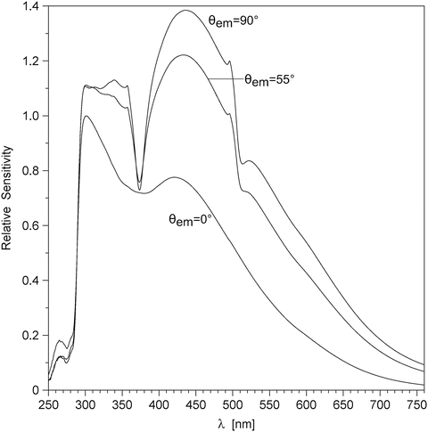
Fig. 3
Spectral sensitivity variation for SLM-48000S spectrofluorometer equipped with Glan–Thompson polarizers, MC-200 monochromators, and R-926 photomultipliers in the emission light path. θ em is the angle of the polarizer, measured from the vertical. Wood’s anomalies are observed near λ = 373 nm and λ = 505 nm with θ em = 90° and θ em = 55°, but not with θ em = 0°, because in the latter case the polarization (electric vector) is parallel to the grooves on the diffraction grating
4.
Spectral correction. It must be emphasized that the spectral sensitivity curve of every fluorescence spectrometer depends on the orientation of the polarizer in the emission light path and on the width of the emission monochromator slits. The spectral sensitivity curve for θ em = 0 and 4-nm monochromator slits is obtained using thermal radiation with the spectral distribution close to that of a blackbody of a known color temperature near 3,000 K. The source of the thermal radiation must have a quartz bulb. The best choice is a tungsten band lamp calibrated at the National Bureau of Standards; if this is not available or does not fit in the cell compartment, then the second-best choice is a miniature 12 V 20 W halogen lamp with a G-4 base, RadioShack catalog number 272-1177, powered by a regulated 16.5 V DC power supply. The lamp is placed in the well that normally houses a fluorescence cell. The band lamp is oriented so that the tungsten band is normal to the axis of the emission optical path. The miniature halogen lamp is oriented so that the axis of the spiral tungsten filament is parallel to the axis of the emission optical path. The lamp holder is sturdy and allows translational alignment in two directions normal to the axis of the emission optical path. The lamp is aligned to maximize the signal from the photomultiplier that normally measures fluorescence emission intensity. A technical spectrum of the lamp is recorded from 250 to 800 nm at 1-nm steps. The technical spectrum is then divided by the blackbody radiation spectrum to obtain the spectral sensitivity curve. The blackbody radiation spectrum is calculated as
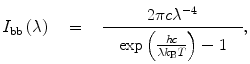
(9)
2.3 Absorption Spectrum
The absorption spectrum is scanned in the wavelength range from 280 to 480 nm or wider. The wavelength step should be 1 nm or a fraction of 1 nm, so that the computer file would contain the value of the absorbance (a.k.a. optical density) at every integer wavelength from 280 to 480 nm. Any UV–VIS spectrophotometer can be used for this purpose. If the spectrophotometer contains two cell holders, one for the “sample” cell and one for the “reference” cell, then the “reference” cell is left empty, because the absorption spectrum is to be used for the inner-filter correction (see Note 6). The absorption spectrum is usually measured after all time-resolved and steady-state fluorescence measurements. If there is a suspicion that the protein molecules may aggregate during the lengthy fluorescence measurements, then the absorption spectrum of the protein cell is measured twice, both before and after fluorescence measurements. With aggregation the absorption spectrum acquires a tail at λ > 315 nm, where none of the 20 protein amino acids absorb radiation. The tail represents the radiation losses due to scattering, and its spectral shape can be mathematically described by the function 1/λ 4. Fluorescence emission from aggregated proteins is always heterogeneous, as well as fluorescence emission from proteins having more than one Trp residue in the amino acid sequence.
3 Computational Procedures
The experimental data obtained as described above need to be processed by a number of computer programs, with each program using a specific algorithm and intended to perform a specific task. The computer programs can be obtained from the author of this chapter. All programs run under Linux operating system on computers with Intel i686 processors and require four shared object libraries, libm.so.6, libgcc_s.so.1, libc.so.6, and libgfortran.so.3, the former three of which are standard components of any Linux operating system, while the fourth one can be easily installed from the Internet. The programs, Linux operating system, and the additional libraries are free. Below each program is described together with the underlying math.
3.1 Correcting and Smoothing Steady-State Spectra
1.
Correction. Technical steady-state emission spectrum should be corrected for the spectral sensitivity variation of the instrument and for the secondary inner-filter effect (the primary inner-filter effect changes the absolute intensity but not the shape of the emission spectrum). The program correct corrects for the spectral sensitivity variation and, if necessary, may also correct for the secondary inner-filter effect using the following recipe:
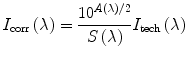
(10)
Here I tech(λ) and I corr(λ) are the technical and the corrected spectrum, A(λ) is the gross absorbance (optical density) spectrum of the same solution in the same cell, and S(λ) is the spectral sensitivity curve of the steady-state fluorescence spectrometer obtained for θ em = 0 and 4-nm monochromator slits.
2.
Smoothing. An experimental steady-state emission spectrum always contains random noise. High-frequency random noise, if it is not removed from the spectrum, will translate into “fine structure” in the functions F λ (λ,t) and F v (v,t), which will hinder the calculation of the FWHM, peak position, etc., and make the results useless. Removal of the high-frequency noise is accomplished by fitting a smooth analytical function to the corrected experimental spectrum. Before the fitting, it is necessary to visually inspect the corrected experimental spectrum and to pick a cutoff wavelength to the right of the scattered excitation light peak but to the left of the shortest wavelength at which TCSPC data were collected (usually 300 nm). The optimum cutoff wavelength is shown by an arrow in Fig. 4. The data at wavelengths shorter than the cutoff wavelength are not used in the fitting. The fitting function must have a number of fitting parameters that can be varied from just 3 (Gaussian) or 5 (skewed Gaussian) to 20 or more depending on the complexity of the spectral shape. The most general fitting function of this type is
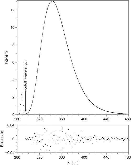
Fig. 4
Corrected spectrum of fluorescence emission from Trp residues in E21W variant of IIAGlc protein at +5 °C, excited at 288.5 nm; this spectrum was used to generate the time-resolved emission spectra published in [2]. This figure illustrates an intermediate step in the data processing, and it was not included in [2]. Main panel: corrected experimental data are depicted by dots; the solid line represents the best fit with the model function in Eq. 11 and m = 10. The fitting was done by the program exppolnu. The arrow points to the cutoff wavelength, which is selected to the right of the scattered light peak and to the left of λ=300 nm, the shortest wavelength at which TCSPC data are collected. The data to the left of the cutoff wavelength are not used in the fitting. The bottom panel shows the residuals (the differences between the data and the fit) on a 40-fold expanded vertical scale. If the residuals are not random (the dots seem to form a wave), then the value of m needs to be increased
(11)
This function is actually an exponential of a polynomial of v, where v = λ −1. The choice of v rather than λ for the argument of the polynomial function is dictated by the fact that the vibrational structure in electronic spectra has a constant period on the v scale, but not on the λ scale. The degree of the polynomial equals m. The number of free fitting parameters a n equals m + 1. For m = 2 the function in Eq. 11 represents a symmetrical Gaussian on the wavenumber scale. For m = 4 it represents a skewed Gaussian. The fitting of the model function in Eq. 11 to the corrected fluorescence emission spectrum is done using the program exppolnu. For Trp residues in proteins, the value of m = 10 always gives a perfect fit. In Fig. 4 the corrected emission spectrum is shown by dots, the best fit by the model function in Eq. 11 with m = 10 is shown by the solid line. The magnified residuals are shown in the bottom panel.
3.2 Combining TCSPC Data
1.
Combining multiple TCSPC data sets. TCSPC data from the right and the left wing of the instrument shown in Fig. 1 need to be added together before the data analysis. The time scale (the time per one MCA channel) is always kept the same for both wings, but the position of the IRF peak may be different, which needs to be taken into account when the TCSPC data are combined. Furthermore, the IRF peak in each wing may shift by as much as ten MCA channels during a 5-h experiment. For this reason, long data collections are always split in parts not exceeding 300 s in duration and the data are saved in different files. The data obtained back-to-back from the same wing, the data from different wings, and the data from similar experiments conducted on different days are combined using the program comb_tcp. The underlying algorithm combines two TCSPC data sets each time it is invoked. If the number of TCSPC data sets exceeds two, then the algorithm is invoked more than once (the algorithm can be invoked any number of times during one run of the program comb_tcp). During the first invocation, data sets 1 and 2 are combined. During the second invocation, the combination of sets 1 and 2 is combined with set 3. During the third invocation, the combination of sets 1, 2, and 3 is combined with set 4. This is repeated until all data sets are combined. The final result is independent of the order in which the data sets are combined.
2.
Get Clinical Tree app for offline access
Algorithm for combining two TCSPC data sets. A TCSPC data set consists of a decay curve, which will be denoted D m (i), and the IRF, which will be denoted E m (i). The IRF is measured quasi-simultaneously with the corresponding decay curve using a Ludox scatterer cell. Both D m (i) and E m (i) are integer-valued functions of the integer variable i, which represents MCA channel number, whereas m denotes the number of the set. For notation simplicity it will be assumed that two sets with m = 1 and m = 2 are being added. The algorithm starts by calculating the correlation function: