(1)
Department of Mathematics, University of Florida, Gainesville, FL, USA
7.1 Introduction
In Chap. 2, we introduced the basic SIR and SIS models and developed tools and techniques for their analysis. In Chap. 5, we saw that incorporating more realism into the models leads to more complex epidemic models with multiple compartments. The mathematical tools developed for the global analysis of the SIS and SIR models are unsuitable for models of dimension three or greater. For instance, the Dulac criterion, used to rule out oscillations, and Bendixon’s theorem can be applied only to planar systems and are not valid in higher dimensions. In this chapter, we develop new tools that are applicable to any number of dimensions.
Much of the local analysis that we performed for the SIR model can be performed for higher-dimensional systems. That is, we again have to look at equilibria, which are classified into a disease-free equilibrium and endemic equilibria, and then consider the linearization around those equilibria by evaluating the Jacobian J. For higher-dimensional systems, the principle for showing stability, namely that all eigenvalues of the characteristic equation
 have negative real parts or are negative, still holds. This is guaranteed by the Hartman–Grobman theorem [155] and by the fact that zero is an asymptotically stable solution of a linear system with constant coefficients if and only if all eigenvalues have negative real part [28]. These results hold for multidimensional systems of ODEs.

7.2 Local Analysis of the SEIR Model
We illustrate the analysis, which is somewhat more elaborate, on the SEIR model. The SEIR model is another classical epidemiological model, which incorporates a compartment of exposed individuals, E(t), where the individuals are infected but not infectious. With S(t) denoting the number of susceptible individuals, I(t) the number of infectious individuals, and R(t) the number of recovered individuals, the model takes the form
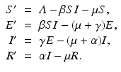
To determine the equilibria of this model, we set the derivatives equal to zero and solve the system
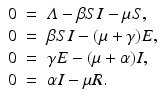
This system has a disease-free equilibrium, which is obtained by setting I = 0,  . To find the endemic equilibria, we solve for E in the third equation,
 and we substitute into the second equation to obtain
 Hence
Hence
 From the first equation, we have


(7.1)

(7.2)
 . To find the endemic equilibria, we solve for E in the third equation,


We define the basic reproduction number as

The reproduction number is positive; it is zero if there is no transmission, that is, β = 0, and it can be interpreted as the number of secondary cases. In particular, we can see that  is the number of susceptible individuals in a disease-free population,
  is the number of secondary cases produced by one infectious individual during its lifespan as infectious, and
  is the fraction of new infections that survive the exposed period and actually become infectious.

(7.3)
 is the number of susceptible individuals in a disease-free population,
  is the number of secondary cases produced by one infectious individual during its lifespan as infectious, and
  is the fraction of new infections that survive the exposed period and actually become infectious.
From the reproduction number, we have the following result:
Proposition 7.1.
The system has a unique disease-free equilibrium  . If
. If  , where

 . If
. If  , where
To investigate the local stability, we consider the Jacobian of the system (7.1). We have

To determine the local stability of the disease-free equilibrium, we evaluate the Jacobian at  :
:

Subtracting  along the main diagonal, we see that the characteristic equation
  has two roots equal to −μ. The remaining roots are the solution to the following equation:

This leads to the following quadratic characteristic equation:
 From here, it is not hard to see that this equation has one positive real root if
  . This leads to the following classical result regarding the disease-free equilibrium.

(7.4)
 :
:
(7.5)
 along the main diagonal, we see that the characteristic equation
  has two roots equal to −μ. The remaining roots are the solution to the following equation:
(7.6)

 . This leads to the following classical result regarding the disease-free equilibrium.
Proposition 7.2.
If  , then the disease-free equilibrium
  is locally asymptotically stable. If
  , we evaluate the Jacobian at the endemic equilibrium. We obtain the following characteristic equation:

Expanding by the last column, we see that the characteristic equation has one root equal to −μ. The remaining roots are solutions to the following equation:

Expanding the determinant, we have, after some simplification, the following polynomial characteristic equation:
![$$\displaystyle{ [\beta I^{{\ast}} +\mu +\lambda ][\mu +\gamma +\lambda ][\mu +\alpha +\lambda ] =\beta S^{{\ast}}\gamma (\mu +\lambda ). }$$](/wp-content/uploads/2016/11/A304573_1_En_7_Chapter_Equ9.gif)
One approach here to showing that all solutions to the above equation have negative real parts is to use the Routh–Hurwitz criterion (Chap. 5). We will apply a somewhat trickier but faster method to establish the same result. The question is whether the above equation has solutions with nonnegative real part. Assume that there is a  with nonnegative real part,
  . Then, we can divide by
  and take the absolute value of both sides of the equation. We have

Recall the value of S ∗. Hence, we have
 From the left-hand side in Eq. (7.10), we have that
 real or complex, as long as
  . If
. If  , where i is the imaginary unit, then
 with
with  , the left-hand side of Eq. (7.10) is always grater than the right-hand side. Hence, the characteristic equation cannot have such solutions. We have established the following result:
 , then the disease-free equilibrium
  is locally asymptotically stable. If
  , we evaluate the Jacobian at the endemic equilibrium. We obtain the following characteristic equation:
(7.7)

(7.8)
![$$\displaystyle{ [\beta I^{{\ast}} +\mu +\lambda ][\mu +\gamma +\lambda ][\mu +\alpha +\lambda ] =\beta S^{{\ast}}\gamma (\mu +\lambda ). }$$](/wp-content/uploads/2016/11/A304573_1_En_7_Chapter_Equ9.gif)
(7.9)
 with nonnegative real part,
  . Then, we can divide by
  and take the absolute value of both sides of the equation. We have
(7.10)

 real or complex, as long as
  . If
. If  , where i is the imaginary unit, then
 with
with  , the left-hand side of Eq. (7.10) is always grater than the right-hand side. Hence, the characteristic equation cannot have such solutions. We have established the following result:
Proposition 7.3.
Assume  is locally asymptotically stable.
 is locally asymptotically stable.
 7.3 Global Stability via Lyapunov Functions
For higher-dimensional systems, there are several techniques that could establish the global stability of an equilibrium. One of the most commonly used is the Lyapunov function. Lyapunov functions are scalar functions that may be used to prove the global stability of an equilibrium. They are named after the Russian mathematician Aleksandr Mikhailovich Lyapunov, who proposed the theory in his doctoral dissertation [98].
7.3.1 Lyapunov–Kasovskii–LaSalle Stability Theorems
Let x ∗ be an equilibrium of x′ = f(x), where f: R n → R n .
Definition 7.1.
A scalar function V (x) such that V: R n → R is called radially unbounded if


One significant property of Lyapunov functions is that they are positive definite in the entire space.
Definition 7.2.
Let V be a continuous scalar function, that is,
 The function V is called positive definite on the entire space if

V (x ∗) = 0,
V (x) > 0 for x ≠ x ∗,
where x ∗ is an equilibrium of the autonomous system x′ = f(x). We define the derivative of V (x) along the solutions of the system of differential equations as


Now we can state Lyapunov’s theorem for global stability of the equilibrium x ∗. For a proof of Lyapunov’s, theorem see [41].
Theorem 7.1 (Lyapunov’s Stability Theorem).
If a function V (x) is globally positively definite and radially unbounded, and its time derivative is globally negative,
 then the equilibrium x ∗ is globally stable.

Definition 7.3.
If a function V (x) exists that satisfies the conditions of Theorem 7.1, then this function is called a Lyapunov function.
There are no established rules for finding a Lyapunov function, and often finding a Lyapunov function is tricky and computationally intensive (but see [146]). However, if a Lyapunov function is found, it can establish the global stability of an equilibrium.
Lyapunov’s Theorem requires that the derivative of a Lyapunov function with respect to t be strictly negative; however, we can often show only nonpositivity. In this case, an extension of Lyapunov’s theorem was given by LaSalle [93] and Krasovskii [91].
Theorem 7.2 (Krasovkii–LaSalle Theorem).
Consider the autonomous system x′ = f(x), where x ∗ is an equilibrium, that is, f(x ∗ ) = 0. Suppose there exists a continuously differentiable function V: R n → R and that this function is positive definite on the entire space and radially unbounded and that it satisfies
 Define the invariant set
 If
If  contains only the equilibrium x ∗ , then the equilibrium x ∗ is globally stable.


 contains only the equilibrium x ∗ , then the equilibrium x ∗ is globally stable.
 7.3.2 Global Stability of Equilibria of the SEIR Model
We illustrate the application of Lyapunov’s theorem by showing global stability of the disease-free equilibrium and the endemic equilibrium for the SEIR model in (7.1).
Proposition 7.4.
Assume  . Then the disease-free equilibrium is globally asymptotically stable.
 . Then the disease-free equilibrium is globally asymptotically stable.
 Proof.
We approach the problem by constructing a Lyapunov function. We will consider the SEIR model on the space of the first three variables only (S, E, I). It is clear that if the disease-free equilibrium for the first three equations is globally stable, then R(t) → 0, and the disease-free equilibrium for the full SEIR model is globally stable.
Consider the following candidate for a Lyapunov function on R + 3. It is sufficient to work with R + 3, because we are interested in working with only the positive orthant.

where κ > 0 is to be determined and  . First, it is not hard to see that V = 0 at the disease-free equilibrium. To establish that V > 0 for all
  , it is enough to notice that
 achieves a global minimum at x = 1 and g(1) = 0. Hence g(x) > 0 for all x > 0 and x ≠ 1. So the first term is positive. The remaining two terms are also clearly positive. The coefficients of E and I are chosen in such a way that the negative term in the E′ equation cancels with the positive term in the I′ equation in (7.1). Furthermore, V is also clearly radially unbounded. We take the derivative of V with respect to t:
![$$\displaystyle{ \begin{array}{ll} \dfrac{d} {dt}V & =\kappa \left (1 -\dfrac{S^{{\ast}}} {S} \right )S'+ \dfrac{1} {\mu +\gamma }E'+\dfrac{1} {\gamma } I' \\ & =\kappa \left (1 -\frac{S^{{\ast}}} {S} \right )\left [\varLambda -\beta SI -\mu S\right ]+ \frac{1} {\mu +\gamma }(\beta SI-(\mu +\gamma )E)+\frac{1} {\gamma } (\gamma E-(\mu +\alpha )I) \\ & = 2\kappa \varLambda -\beta \kappa SI -\kappa \mu S-\frac{\varLambda ^{2}\kappa } {\mu S}+\frac{\varLambda \beta \kappa } {\mu }I+ \frac{\beta } {\mu +\gamma }SI -\frac{\mu +\alpha } {\gamma } I, \end{array} }$$](/wp-content/uploads/2016/11/A304573_1_En_7_Chapter_Equ13.gif)
where after differentiation, we have used equations (7.1) to replace the derivatives with the right-hand sides. The last line is obtained by multiplying out. We have several positive terms for which we need to compensate. If we choose  , then the S I terms have the same coefficient and opposite signs, so they cancel each other. We combine the two I-terms and the remaining terms as follows:

Since  , the last term is nonpositive. The first term is more interesting. If we set
  , then we have
  . We claim that this expression is positive for every a > 0, a ± 1 indeed,
![$$\displaystyle{a + \frac{1} {a} - 2 = \frac{a^{2} - 2a + 1} {a} = \frac{(a - 1)^{2}} {a} > 0.}$$
” src=”/wp-content/uploads/2016/11/A304573_1_En_7_Chapter_Equq.gif”></DIV></DIV></DIV>Hence we have <SPAN class=EmphasisTypeItalic>V</SPAN> ′ < 0 for all (<SPAN class=EmphasisTypeItalic>S</SPAN>, <SPAN class=EmphasisTypeItalic>E</SPAN>, <SPAN class=EmphasisTypeItalic>I</SPAN>) ≠ (<SPAN class=EmphasisTypeItalic>S</SPAN> <SUP>∗</SUP>, 0, 0). Therefore, by Lyapunov’s theorem, the disease-free equilibrium is globally asymptotically stable. □ </DIV></DIV><br />
<DIV class=Para>Now we consider the endemic equilibrium. The endemic equilibrium is unique and locally stable whenever it exists. For <SPAN id=IEq36 class=InlineEquation><IMG alt=]() 1$$
” src=”/wp-content/uploads/2016/11/A304573_1_En_7_Chapter_IEq36.gif”>, the only other equilibrium is
1$$
” src=”/wp-content/uploads/2016/11/A304573_1_En_7_Chapter_IEq36.gif”>, the only other equilibrium is  , which is unstable. This suggests that the endemic equilibrium may be globally stable. Indeed, that is the case. The global stability of the endemic equilibrium for the SEIR model was first established by Li and Muldowney [96] using different techniques. The global stability of the endemic equilibrium of the SEIR model via a Lyapunov function was fist established by Korobeinikov and Maini [89]. We will establish this result via a Lyapunov function. Before we state the main result, we include a lemma that is very helpful in establishing the negativity of the time derivative of a candidate Lyapunov function.
Get Clinical Tree app for offline access


(7.12)
 . First, it is not hard to see that V = 0 at the disease-free equilibrium. To establish that V > 0 for all
  , it is enough to notice that
 achieves a global minimum at x = 1 and g(1) = 0. Hence g(x) > 0 for all x > 0 and x ≠ 1. So the first term is positive. The remaining two terms are also clearly positive. The coefficients of E and I are chosen in such a way that the negative term in the E′ equation cancels with the positive term in the I′ equation in (7.1). Furthermore, V is also clearly radially unbounded. We take the derivative of V with respect to t:
![$$\displaystyle{ \begin{array}{ll} \dfrac{d} {dt}V & =\kappa \left (1 -\dfrac{S^{{\ast}}} {S} \right )S'+ \dfrac{1} {\mu +\gamma }E'+\dfrac{1} {\gamma } I' \\ & =\kappa \left (1 -\frac{S^{{\ast}}} {S} \right )\left [\varLambda -\beta SI -\mu S\right ]+ \frac{1} {\mu +\gamma }(\beta SI-(\mu +\gamma )E)+\frac{1} {\gamma } (\gamma E-(\mu +\alpha )I) \\ & = 2\kappa \varLambda -\beta \kappa SI -\kappa \mu S-\frac{\varLambda ^{2}\kappa } {\mu S}+\frac{\varLambda \beta \kappa } {\mu }I+ \frac{\beta } {\mu +\gamma }SI -\frac{\mu +\alpha } {\gamma } I, \end{array} }$$](/wp-content/uploads/2016/11/A304573_1_En_7_Chapter_Equ13.gif)
(7.13)
 , then the S I terms have the same coefficient and opposite signs, so they cancel each other. We combine the two I-terms and the remaining terms as follows:
(7.14)
 , the last term is nonpositive. The first term is more interesting. If we set
  , then we have
  . We claim that this expression is positive for every a > 0, a ± 1 indeed,
 , which is unstable. This suggests that the endemic equilibrium may be globally stable. Indeed, that is the case. The global stability of the endemic equilibrium for the SEIR model was first established by Li and Muldowney [96] using different techniques. The global stability of the endemic equilibrium of the SEIR model via a Lyapunov function was fist established by Korobeinikov and Maini [89]. We will establish this result via a Lyapunov function. Before we state the main result, we include a lemma that is very helpful in establishing the negativity of the time derivative of a candidate Lyapunov function.
Lemma 7.1.
Assume that  are n positive numbers. Then their arithmetic mean is greater than or equal to their geometric mean. In particular,

 are n positive numbers. Then their arithmetic mean is greater than or equal to their geometric mean. In particular,
Theorem 7.3.
Assume ![$$\mathcal{R}_{0} > 1$$
” src=”/wp-content/uploads/2016/11/A304573_1_En_7_Chapter_IEq39.gif”></SPAN> <SPAN class=EmphasisTypeItalic>. Then the endemic equilibrium is globally asymptotically stable.</SPAN> </DIV></DIV><br />
<DIV class=]()
Proof.
We consider again only the first three components of system (7.1), (S, E, I). We assume that they belong to the positive orthant R + 3. We define a Lyapunov function

where κ 1 > 0, κ 2 > 0, and κ 3 > 0 will be determined later. Notice that V = 0 when (S, E, I) = (S ∗, E ∗, I ∗) and V > 0 otherwise; V is also radially unbounded. What remains to be proved is that the derivative of V with respect to t is negative. We differentiate with respect to t and replace S′, E′, and I′ with their equals from (7.1):


(7.15)

(7.16)
One of the classical first steps here is to replace  with its equal from the equilibrium equations, that is,
  . Then μ S ∗−μ S can be combined with the first term in the product to yield a negative term. We multiply out all other products:

Now we can see that if κ 1 = κ 2, then −κ 1 β S I can be canceled with κ 2 β S I. Also, where we have fractions, we multiply and divide by the equilibrium value:

We want to combine all constant terms with all fractional terms, because all constant terms are positive, and all fractional terms are negative. First, we notice that since κ 1 = κ 2, we have  from the corresponding equilibrium equation. We need to choose κ 3 such that
 Hence,
  . We pull out κ 1 β S ∗ I ∗ from all terms. We have
![$$\displaystyle\begin{array}{rcl} \frac{dV } {dt} =& -& \kappa _{1}\frac{(S - S^{{\ast}})^{2}} {S} +\kappa _{1}\beta S^{{\ast}}I^{{\ast}}\left [3 -\frac{S^{{\ast}}} {S} - \frac{E^{{\ast}}SI} {ES^{{\ast}}I^{{\ast}}} -\frac{I^{{\ast}}E} {IE^{{\ast}}}\right ] \\ & +& (\kappa _{1}\beta S^{{\ast}}-\kappa _{ 3}(\mu +\alpha ))I + (\kappa _{3}\gamma -\kappa _{2}(\mu +\gamma ))E. {}\end{array}$$](/wp-content/uploads/2016/11/A304573_1_En_7_Chapter_Equ19.gif)
Because  , the last two terms in the formula above are zero. We may now choose
  . Then
 In this case, the derivative of the Lyapunov function becomes
![$$\displaystyle{ \frac{dV } {dt} = -\frac{(S - S^{{\ast}})^{2}} {S} +\beta S^{{\ast}}I^{{\ast}}\left [3 -\frac{S^{{\ast}}} {S} - \frac{E^{{\ast}}SI} {ES^{{\ast}}I^{{\ast}}} -\frac{I^{{\ast}}E} {IE^{{\ast}}}\right ]. }$$](/wp-content/uploads/2016/11/A304573_1_En_7_Chapter_Equ20.gif)
The first term above is clearly negative unless S = S ∗. We argue that the second term is also negative. Indeed, we will apply Lemma 7.1. Let
 Then, notice that x 1 x 2 x 3 = 1. According the the lemma, the arithmetic mean is larger than the geometric mean. Therefore,
 Hence, the second term is nonpositive, and it is zero whenever (S, E, I) = (S ∗, E ∗, I ∗). We have
 We now have to apply the Krasovkii–LaSalle theorem. We consider the set where the Lyapunov function is equal to zero:
 It is clear that V ′ = 0 if and only if
 Since S = S ∗, then
  , and from the first equation in system (7.1), we can conclude that I = I ∗. Finally, from the second equality above, we have
 It is easy to see that this equality holds if and only if E = E ∗. Hence, the set
  consists of the singleton (S ∗, E ∗, I ∗). This concludes the proof. □
 with its equal from the equilibrium equations, that is,
  . Then μ S ∗−μ S can be combined with the first term in the product to yield a negative term. We multiply out all other products:
(7.17)

(7.18)
 from the corresponding equilibrium equation. We need to choose κ 3 such that
 . We pull out κ 1 β S ∗ I ∗ from all terms. We have
![$$\displaystyle\begin{array}{rcl} \frac{dV } {dt} =& -& \kappa _{1}\frac{(S - S^{{\ast}})^{2}} {S} +\kappa _{1}\beta S^{{\ast}}I^{{\ast}}\left [3 -\frac{S^{{\ast}}} {S} - \frac{E^{{\ast}}SI} {ES^{{\ast}}I^{{\ast}}} -\frac{I^{{\ast}}E} {IE^{{\ast}}}\right ] \\ & +& (\kappa _{1}\beta S^{{\ast}}-\kappa _{ 3}(\mu +\alpha ))I + (\kappa _{3}\gamma -\kappa _{2}(\mu +\gamma ))E. {}\end{array}$$](/wp-content/uploads/2016/11/A304573_1_En_7_Chapter_Equ19.gif)
(7.19)
 , the last two terms in the formula above are zero. We may now choose
  . Then
![$$\displaystyle{ \frac{dV } {dt} = -\frac{(S - S^{{\ast}})^{2}} {S} +\beta S^{{\ast}}I^{{\ast}}\left [3 -\frac{S^{{\ast}}} {S} - \frac{E^{{\ast}}SI} {ES^{{\ast}}I^{{\ast}}} -\frac{I^{{\ast}}E} {IE^{{\ast}}}\right ]. }$$](/wp-content/uploads/2016/11/A304573_1_En_7_Chapter_Equ20.gif)
(7.20)


 , and from the first equation in system (7.1), we can conclude that I = I ∗. Finally, from the second equality above, we have
 consists of the singleton (S ∗, E ∗, I ∗). This concludes the proof. □
 7.4 Hopf Bifurcation in Higher Dimensions
The Hopf bifurcation theorem that we stated in Chap. 3 is valid in higher dimensions. We will use it here without restating it. The characteristic equation of higher-dimensional ODE systems is a polynomial equation of degree n. The Hopf bifurcation theorem requires that for some value of a parameter, this equation have a purely imaginary root and all other roots have negative real part. The following theorem gives a necessary and sufficient condition for this to happen [57]:
Theorem 7.4.
Let  , where
  , be a polynomial of degree n with real coefficients:
 with a 0 > 0. Let
  be the Hurwitz determinants for the polynomial
  . Then
  has a pair of distinct roots, − iω and iω, on the imaginary axis, and all other roots are in the left half-plane if and only if
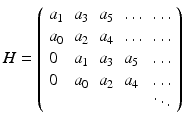
is called a Hurwitz matrix. The ith-order principal minor of H is called the ith Hurwitz determinant Δ i .
 , where
  , be a polynomial of degree n with real coefficients:
 be the Hurwitz determinants for the polynomial
  . Then
  has a pair of distinct roots, − iω and iω, on the imaginary axis, and all other roots are in the left half-plane if and only if
(7.21)
To illustrate Hopf bifurcation in higher dimensions, we consider a specific example that focuses on recurrent outbreaks in childhood disease. It has been long since observed that the incidence of some childhood diseases like measles and chickenpox experiences oscillations [130]. The question whether these oscillations can be captured by an autonomous ODE model was first investigated by Feng and Thieme [61], who considered an SIQR model to approach the problem. To introduce the model, let S(t), I(t), Q(t), and R(t) be the numbers of susceptible, infected/infectious, isolated, and recovered individuals. We assume that isolated individuals do not mix in the population, and we define the active population  . The total population as usual is denoted by N(t). The model is as follows:
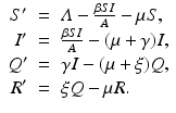
The model assumes that the isolation is perfect, that is, that everybody who becomes infectious is isolated and that isolated individuals cannot infect. We will show that the endemic equilibrium of this model is not always stable, but it can undergo a Hopf bifurcation that leads to a stable oscillatory solution. That, in particular, means that the endemic equilibrium is not globally stable.
 . The total population as usual is denoted by N(t). The model is as follows:
(7.22)
It is not hard to see that the model has two equilibria: a disease-free equilibrium  and an endemic equilibrium
  . To obtain the endemic equilibrium, we introduce the fractions
  ,
,  ,
,  , and
, and  . Clearly,
  and
and

 and an endemic equilibrium
  . To obtain the endemic equilibrium, we introduce the fractions
  ,
,  ,
,  , and
, and  . Clearly,
  and
and
The endemic equilibrium is a solution of the following system:
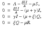
With the new notation, the last three equations from the system become

Hence,

From the first equation in (7.23), we have (recall  )
)
 Subtracting Q ∗ from both sides, we have
 Dividing by the left-hand side, we have
 We replace s and q from (7.25) and solve for i to obtain
 and
and
 where
where  is the reproduction number of the disease. Define
  . Then from
  , we have

(7.23)

(7.24)

(7.25)
 )
)


 is the reproduction number of the disease. Define
  . Then from
  , we have


