(1)
Department of Mathematics, University of Florida, Gainesville, FL, USA
12.1 Introduction
Chronological age is perhaps one of the most important factors distinguishing individuals in a population that needs to be incorporated in population and epidemic models. Undoubtedly, vital characteristics such as birth and death rates differ markedly among the individuals of various ages. Age is also a key to capturing important mixing patterns in epidemic models. For instance, in childhood diseases, children predominantly mix with other children in similar age groups as well as with the individuals of the age groups of their parents and grandparents. Children are at greatest risk for contracting malaria and exhibiting strongest symptoms and highest death rate, yet malaria affects all age groups. Incidence of HIV is highest in the age groups from age twenty to age forty-five. Endemic models that incorporate births and deaths should also preferably incorporate age structure, since with time, the age profile of the population may change, and that may affect the dynamics of the disease.
Age-structured epidemic models are built on the basis of age-structured population models. There are several excellent introductory texts for age-structured population models [78, 46]. For completeness, we will introduce here first the linear age-structured population model. Most epidemic models use the linear model as a baseline population model.
12.2 Linear Age-Structured Population Model
The Malthusian model, which is also linear, considers a homogeneous population in which individuals are not distinguished by age [104]. The linear age-structured model is a strict analogue of the Malthusian model but allows for variability in age. As in the Malthusian model, the age-structured model considers a single population, not stratified by sex, which is isolated (no emigration and immigration) and lives in an invariant habitat, that is, the birth and death rates can be assumed time-independent. The only characteristics by which individuals in the population differ is age.
Models that structure the population by age can be continuous or discrete. In this chapter, we will consider the continuous age-structured model. Because age and time are considered two independent variables, the resulting continuous models are cast as partial differential equation models. It was the physician A.G. McKendrick who first considered an age-structured PDE model for the dynamics of a one-sex population [115]. Earlier age-structured models were developed by Sharpe and Lotka [144, 3] but they were formulated as integral equations of Volterra type. We will first introduce McKendrick’s age-structured PDE model, and then derive Lotka’s model.
12.2.1 Derivation of the Age-Structured Model
McKendrick model introduces two independent variables: age a and time t. The distribution of the female population can be described by a function u(a, t) that denotes the age-density of individuals at age a at time t. We assume a ∈ [0, a †], t ≥ 0, where  denotes the maximal age, which may be assumed infinite. If
  , then we assume that u(a, t) = 0 for all sufficiently large values of a. The function gives “density” rather than numbers, because the number of individuals of ages between a and a +Δ A, where Δ a is a small increment, at time t is approximately u(a, t)Δ a. Thus, the total number of individuals of ages in the interval [a 1, a 2] at time t is given by the integral
 Respectively, the total number of individuals in the population or the total population size at time t is given by
 Consider a cohort of individuals, that is, a group of individuals of age in an interval of length Δ a. The number of individuals in that cohort is u(a, t)Δ a. If a small interval of time Δ t elapses, then those individuals who where of age a at time t will be of age a +Δ t, and time is t +Δ t. The number of these individuals is u(a +Δ t, t +Δ t)Δ a. This is the same cohort. Their new number, however, is smaller than their original number, since some of these individuals will have died. We assume that the members of the population leave the population only by death. We denote the age-specific per capita mortality rate by μ(a). Then the number of individuals that die at age [a, a +Δ a] at time t is μ(a)u(a, t)Δ a. For the whole interval of time Δ t, that number would be
  . The balance law can be written as

 denotes the maximal age, which may be assumed infinite. If
  , then we assume that u(a, t) = 0 for all sufficiently large values of a. The function gives “density” rather than numbers, because the number of individuals of ages between a and a +Δ A, where Δ a is a small increment, at time t is approximately u(a, t)Δ a. Thus, the total number of individuals of ages in the interval [a 1, a 2] at time t is given by the integral

 . The balance law can be written as
(12.1)
Dividing both sides by Δ a Δ t, we obtain a difference quotient on the left-hand side:

We take the limit as t → 0. If u(a, t) is a differentiable function with respect to each variable, we have
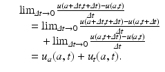
We obtain McKendrick’s equation, also referred to as the McKendrick–von Foerster equation, since it was later derived by von Foerster (1959) in the context of cell biology [63]:


(12.2)

(12.3)

(12.4)
The mortality rate is connected to the probability of survival (Fig. 12.1). Let π(a) be the probability of survival from birth to age a. Suppose we start from a cohort of newborns of size P. Then π(a)P gives the number of individuals from the cohort who are of age a. Similarly, π(a +Δ a)P gives the number of individuals from the cohort who are of age a +Δ a. Then π(a +Δ a)P −π(a)P is the number of individuals who have died in the age interval Δ a. We have
 Canceling P and dividing by Δ a, we have
 Taking the limit as Δ a → 0 and assuming that the probability of survival π(a) is a differentiable function, we obtain the following ordinary differential equation for π(a):
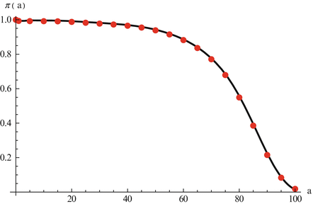


Fig. 12.1
Data on age-specific probability of survival in the United States in 2007. The data are taken from the life tables in the U.S. Vital Statistics Reports [15]. Data are interpolated to show the continuous curve


(12.5)
 is the probability that an individual will survive from age a 1 to age a 2. Age-dependent mortality μ(a) can be found in the national vital statistics files [121], but it is advisable that it be estimated from the life tables and the probability of survival. From the formula (12.5), we have

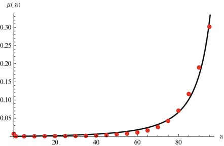
Fig. 12.2
Data on age-specific mortality in the United States in 2007. The data are taken from life tables of the the U.S. Vital Statistics Reports [15] as explained in the text. The age-specific function fitted to the data is 

Remark 12.1.
If  , then we must have
 which means that no one survives until the maximal age. That, in turn, implies that

 , then we must have

Equation (12.4) is a first-order linear partial differential equation. It is defined on the domain
 that is, in the first quadrant. We will need conditions on the boundary of the domain to complete the model. In particular, we need to specify the age density for the initial population distribution at time t = 0:
 where u 0(a) is a given function. The function u 0(a) is called the initial population density. It is assumed that u 0(a) ≥ 0. Furthermore,
 where P 0 is the initial total population size.


The value u(0, t) is the number of newborns at time t. To model the birth process, we introduce the age-specific per capita birth rate β(a). Since there are u(a, t)Δ a females in the population with ages in the interval [a, a +Δ a], it follows that β(a)u(a, t)Δ a gives the number of births to females of age [a, a +Δ a] at time t. Therefore, the total number of births at time t is the sum of all births at all ages:  . Taking the limit as Δ a → 0, we obtain an integral in place of the sum. Thus, the total birth rate is given by
 which also gives the total number of newborns at time t. That is, we have

 . Taking the limit as Δ a → 0, we obtain an integral in place of the sum. Thus, the total birth rate is given by

Data on fertility for the United States in 2010 and a typical form of birth rate are given in Fig. 12.3.
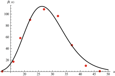

Fig. 12.3
Data on age-specific fertility rate in the United States in 2010. The data are taken from the U.S. Vital Statistics Reports [70]. The age-specific function fitted to the data is 

The full McKendrick–von Foerster age-structured population model takes the form

The condition specified on the boundary a = 0, that is, u(0, t), is called a boundary condition. Since the boundary condition is not specified through a given

(12.6)
function but through an equation that depends on the entire unknown function u(a, t), this boundary condition is referred to as a nonlocal boundary condition. The condition giving a value to u(a, 0) is called an initial condition.
12.2.2 Reformulation of the Model Through the Method of the Characteristics. The Renewal Equation
Model (12.6) can be recast in an integral equation form, a form first derived by Sharpe and Lotka [3, 144]. To obtain the integral equation form, we must integrate the partial differential equation in model (12.6). That can be done through the method of characteristics. The method of characteristics typically applies to first-order hyperbolic partial differential equations. The method identifies curves, called characteristics, along which the partial differential equation reduces to an ordinary differential equation. Then the ordinary differential equation can be integrated from some initial data given on a suitable curve. Finally, the solution of the ordinary differential equation can be transformed into a solution for the original PDE.
An important step in the method of characteristics is identifying the characteristics of the PDE. This is relatively simple for almost linear PDEs. For an almost linear PDE of the form
 in parameterized form, the characteristics are given by

Therefore, in our case we have
 Dividing the one of the equations by the other, we have dt∕da = 1. Hence t = a + c, where c is an arbitrary constant. This implies that the characteristics are lines of slope 1, called characteristic lines of the PDE. What is the practical significance of the characteristic lines? The value of u(a, t) along the characteristic lines models one cohort of individuals. Thus the value of u(a, t) is determined by previous values of u(a, t) along the characteristics, and in particular by the value of u where the characteristic line crosses the boundary of
  .
.


(12.7)

 .
.The integral formulation can be derived from the partial differential equation through a rigorous procedure, called integration along the characteristic lines. To apply the procedure, we fix a point (a 0, t 0) in the first quadrant. We parameterize the characteristic line that goes through that point. If we denote by s the parameter for the fixed point (a 0, t 0) and a variable s, then u(a 0 + s, t 0 + s) gives the value of u along the characteristic line. Define v(s) = u(a 0 + s, t 0 + s). Then the derivative along the characteristic line can be written as
 We let also
  . Then the partial differential equation in model (12.6) can be written as the following ordinary differential equation along the characteristic line:
 This ODE can easily be solved to give

Now we have to interpret this solution in terms of u and two variables a and t. We consider two cases:

 . Then the partial differential equation in model (12.6) can be written as the following ordinary differential equation along the characteristic line:

(12.8)
1.
a 0 ≥ t 0. The solution (12.8) gives, in the original variables,

Now we specify our original point to have been fixed on one of the boundaries. Since we are in the case a 0 ≥ t 0, we must take t 0 = 0. Then s = t and a 0 = a − t. The choice of s and a 0 is made in such a way that a 0 + s = a and t 0 + s = t. With these specifications, from (12.9) we obtain the solution in the case a 0 ≥ t 0, that is, the solution when a ≥ t:


(12.9)

(12.10)
2.
a 0 < t 0. Again

Now we set a 0 = 0. Then s = a, t 0 = t − a. Substituting above, we get for a < t,


(12.11)

So finally, the solution of the PDE can be written in the form

(12.12)
This would have been an explicit solution of the partial differential equation if B(t) were a given function. However, B(t) depends on u(a, t). Thus, this representation is another equation for u(a, t). This representation is not easy to work with, since it is an equation for a function of two variables. It is customary to rewrite this representation in the form of an equation for the function B(t). To do that, we substitute the expression for u(a, t) from (12.12) into the formula for B(t). We have two cases:
Get Clinical Tree app for offline access

Case  :
:


 :
:In this case, we have
 :
:

 :
:In this case, we have only  . Therefore, we have the following equation for B(t):
 . Therefore, we have the following equation for B(t):
(12.14)
where F(t) is a given function:


Equation (12.14) is a linear Volterra integral equation of convolution type with kernel K(a) = β(a)π(a). The function K(a) is sometimes referred to as a maternity function [78]. Equation (12.14) is called the renewal equation or Lotka equation. If we can solve (12.14) and determine B(t) from it, then we can obtain u(a, t) from (12.12).
12.2.3 Separable Solutions. Asymptotic Behavior
The McKendrick–von Foerster model (12.6) is a linear model. Thus its solutions are not necessarily bounded but grow or decay to zero nearly exponentially in time. It can be shown that all solutions approach in time a separable solution. Separable solutions for partial differential equation are solutions that can be written as a product of two functions: a function of age and a function of time, that is, the solution can be written in the form u(a, t) = T(t)ϕ(a). It can be shown (see Problem 12.4) that the time-dependent function T(t) is actually an exponential function. Hence, the separable solutions of the model (12.6) are of the form
 To find the separable solutions, we have to find the number
  and the function ϕ(a). To find
  and ϕ(a), we substitute in the differential equation of model (12.6). Therefore, we have
 where the prime denotes a derivative with respect to a. After canceling
  , we obtain the differential equation for the function ϕ(a):
 This is a first-order linear ordinary differential equation, which can be explicitly solved. The solution is given by
 where the constant ϕ 0 = ϕ(0) is unknown and will be specified later. Hence, we have the following form for the solution u(a, t):
 We seek to satisfy the boundary condition in model (12.6):
 Therefore,
  should be identified in such a way that the equation below is satisfied.

 and the function ϕ(a). To find
  and ϕ(a), we substitute in the differential equation of model (12.6). Therefore, we have
 , we obtain the differential equation for the function ϕ(a):


 should be identified in such a way that the equation below is satisfied.
The characteristic equation of the McKendrick–von Foerster model is


(12.15)
This is a transcendental equation, and it can have multiple solutions for  that are real and complex. It turns out that the Eq. (12.15) has a unique real solution if β(a) is positive on some positive interval:
 that are real and complex. It turns out that the Eq. (12.15) has a unique real solution if β(a) is positive on some positive interval:
The unique real solution  of Eq. (12.15) gives the growth rate of the population for the age-structured model (12.6). It is similar to the population growth rate derived from the Malthusian model.
 of Eq. (12.15) gives the growth rate of the population for the age-structured model (12.6). It is similar to the population growth rate derived from the Malthusian model.
Definition 12.1.
The parameter  is called a Malthusian parameter or growth rate of the population.
 is called a Malthusian parameter or growth rate of the population.
Proof.
Define
 Because
  is a strictly decreasing function of
  . The function
  may not be defined for all values of
  , particularly if
  . Assume that
  is defined and continuous on the interval
  . We have
 Hence, there is a unique real value
  that satisfies
  . □
. □

 is a strictly decreasing function of
  . The function
  may not be defined for all values of
  , particularly if
  . Assume that
  is defined and continuous on the interval
  . We have
 that satisfies
  . □
. □ Stay updated, free articles. Join our Telegram channel

Full access? Get Clinical Tree


![$$\beta (a) \geq \hat{\beta }> 0$$
” src=”/wp-content/uploads/2016/11/A304573_1_En_12_Chapter_IEq20.gif”></SPAN> <SPAN class=EmphasisTypeItalic>for a ∈ [a</SPAN> <SUB>1</SUB> <SPAN class=EmphasisTypeItalic>,a</SPAN> <SUB>2</SUB> <SPAN class=EmphasisTypeItalic>]. Then there is a unique real solution</SPAN> <SPAN id=IEq21 class=InlineEquation><IMG alt=](/wp-content/uploads/2016/11/A304573_1_En_12_Chapter_IEq21.gif)