(10.1)
As such, if we know the value of two of these variables, we will automatically know the value of the third. Consequently, when the true underlying process affecting a dependent variable includes linear effects of some or all of APC, there is a risk that we will pick the wrong combination, given that we could swap a term for the combination of the other two terms without changing the data. For example, take a contrived hypothetical process in which, say, an individual’s level of health is affected by all of age, period and cohort, each with an effect size of 1:

(10.2)

(10.3)

(10.4)
Unfortunately, there is no satisfactory solution to this exact collinearity. The problem is that the collinearity is present in the underlying process that creates the data and therefore in the population as a whole (not just in the sample). This means that neither a more sophisticated model, nor a larger dataset, will solve the problem. However as we see in the next section, a number of solutions to the identification problem have been proposed, many of which fail to understand the impossibility of what they try to do:
The continued search for a statistical technique that can be mechanically applied always to correctly estimate the effects is one of the most bizarre instances in the history of science of repeated attempts to do the logically impossible (Glenn 2005, p. 6).
‘Solutions’ to the APC Identification Problem
The most common ‘solution’, and that suggested first by Mason et al. (1973), is to constrain certain parameters in a model to be equal.2 Thus, each age, period and cohort group is entered into a regression model as a dummy variable, but two groups are combined as if they were a single group. This means that the dependency in Eq. 10.1 no longer applies (that is, it is no longer possible to always be sure of the value of one of the APC variables if you know the value of the other two). However, as Mason et al. recognised (but unfortunately many who use the Mason et al. method do not), solving the dependency in the model does not solve the dependency in the real world (Glenn 1976, 2005; Osmond and Gardner 1989). Whilst the model will produce an answer, there is no way of knowing whether that answer is correct unless we know that the constraint imposed is exactly correct. Thus whilst saying that individuals born in 1960 are substantively the same as those born in 1961 may seem innocuous, such an assumption could have a profound effect on the estimated results, and produce very different results from models using other apparently innocuous assumptions. Crucially, all of these models will have identical model fit statistics, meaning there is no way of choosing one constraint over another without strong prior knowledge. Other models use similar constraints, for example using aggregated groups for one of APC similarly constrains the parameters within those groups, for example see Page et al. (2013). These models are subject to the same problem – the identification problem is merely hidden beneath coarser data. Unless there is very good theory to believe that the groupings imposed are exactly valid, the model will generally fail to produce correct inference.
In recent years more solutions to the identification problem have been proposed.3 This section now focusses on one of these – Yang and Land’s Hierarchical APC (HAPC) model (Yang and Land 2006, 2013).
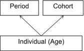
The HAPC model conceptualises period and cohorts as contexts in which individuals (of a given age) reside. This structure makes repeated cross-sectional data (that is survey data with multiple surveys over time) apparently suitable to be modelled with a multilevel cross-classified structure (Browne et al. 2001), whereby individuals are nested within cohort groups and periods of time, but periods are not nested within cohort groups or vice-versa meaning a simple hierarchical structure is not possible (see Fig. 10.1). Thus, the model is specified algebraically as follows:


The dependent variable,  is measured for individuals i in period j1 and cohort j2. The ‘micro’ model has linear and quadratic age terms, with coefficients
  and
and  respectively, a constant that varies across both periods and cohorts, and a level-1 residual error term. The ‘macro’ model defines the intercept in the micro model by a non-varying constant
  , and a residual term for each period and cohort. The period, cohort and level-1 residuals are all assumed to follow Normal distributions, each with variances that are estimated.


(10.5)
 is measured for individuals i in period j1 and cohort j2. The ‘micro’ model has linear and quadratic age terms, with coefficients
  and
and  respectively, a constant that varies across both periods and cohorts, and a level-1 residual error term. The ‘macro’ model defines the intercept in the micro model by a non-varying constant
  , and a residual term for each period and cohort. The period, cohort and level-1 residuals are all assumed to follow Normal distributions, each with variances that are estimated.
Fig. 10.1
Structural diagram of the HAPC model. Individuals, of different ages, are nested within periods, and within a cohort group. This is cross-classified because periods do not nest within cohort groups, nor vice-versa (Adapted from Bell and Jones (2014a) figure 1)
This is an appealing conceptual design: “treating periods and cohort as contexts, and age as an individual characteristic, is intuitive to some degree because we move from one period to another as time passes, and we belong to cohort groups that have common characteristics, whereas aging is a process that occurs within an individual” (Bell and Jones 2014a, p. 340). However, Yang and Land go beyond this, arguing that this model does not incur the identification problem, because (a) the age effect is specified as a quadratic equation, and (b) because the multilevel model treats age differently from periods and cohorts:
the underidentification problem of the classical APC accounting model has been resolved by the specification of the quadratic function for the age effects (Yang and Land 2006, p. 84)
An HAPC framework does not incur the identification problem because the three effects are not assumed to be linear and additive at the same level of analysis (Yang and Land 2013, p. 191)
This contextual approach … helps to deal with (actually completely avoids) the identification problem (Yang and Land 2013, p. 71)
Unfortunately, Yang and Land are misguided in their belief in the HAPC model to do the logically impossible, as simulation studies have shown (Bell and Jones 2014a; Luo and Hodges 2013). Yang and Land’s model can, and has, produced profoundly misleading results. For example, consider Reither, Hauser and Yang’s APC study of obesity in the USA (Reither et al. 2009). They used the HAPC model to find that the recent obesity epidemic is primarily the result of period effects. However, simulations that we conducted (Bell and Jones 2014b) showed that these results could have been found when cohorts rather than periods were behind the increase in obesity. This is shown in Fig. 10.2 – data generated by us with a large cohort effect and no period trend (column 1) produced results suggesting erroneously that period effects were more important (column 2), in line with the results found by Reither et al. (column 3). The difference between these two possible sets of results are important from a policy perspective – a significant cohort trend would suggest that interventions should be targeted at young people in their formative years, whereas a period trend would suggest that interventions would be worthwhile for individuals at all stages of the life course. Additionally, the life course (age) effect found by Reither et al. differed significantly from that proffered by the simulations (row 1 of Fig. 10.2). Once again, failing to appropriately model period and cohort effects can have a big effect on the found life course effect, and vice versa.
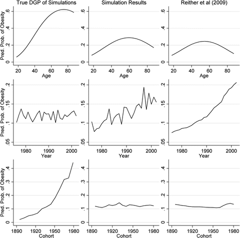

Fig. 10.2
(Column 1) The true data generating process (DGP) of simulated datasets; (column 2) the results from applying the HAPC model to those simulated datasets; and (column 3) the results found by Reither et al. (2009), for the age, period and cohort effects (rows 1, 2 and 3 respectively) (This figure is adapted from figure 1 in Bell and Jones (2014b))
How to Model APC Effects Robustly
Whilst the HAPC model does not work as its authors intended, it does offer a compelling conceptual framework which is useful looking forward to ways one might model age, period and cohort effects together in a single model without falling foul of the identification problem. We have argued from the beginning that discerning APC effects mechanically is impossible. However, if we are willing to make certain assumptions about the nature of those APC effects, then inference is possible, and the HAPC model provides us with a useful framework in which to do so.
These assumptions need to be strong: for example one of the APC trends is often constrained to a certain value. The easiest way to do this is to constrain one of the period and cohort linear trends to zero by including the other as a linear fixed effect. For example, we may be willing to assume that there is no linear period trend, and include a linear cohort fixed effect4 in the model. Thus, Eq. 10.5 is extended to:


We do not need to assume that there is no variation between periods in this model – indeed the period residual term  remains in the model meaning periods (and cohorts) can still have contextual effects. However, we do assume that there is no linear trend over time in the true period residuals, because these will be absorbed by the age and cohort effects in this model.5 If this assumption is justified, such a model will produce correct inference both about the linear age and cohort trends, and about the period and cohort random deviations from those trends (Bell and Jones 2014a). We would argue that often constraining the period trend to zero is a reasonable course of action. For us, the mechanism for long-run change is more easily conceptualised through cohorts than periods – change occurring by influencing people in their formative years rather than ‘something in the air’ that influences all age groups equally and simultaneously. However, this is of course dependent on the research question and subject area, and the researchers own understanding of the process at hand.


(10.6)
 remains in the model meaning periods (and cohorts) can still have contextual effects. However, we do assume that there is no linear trend over time in the true period residuals, because these will be absorbed by the age and cohort effects in this model.5 If this assumption is justified, such a model will produce correct inference both about the linear age and cohort trends, and about the period and cohort random deviations from those trends (Bell and Jones 2014a). We would argue that often constraining the period trend to zero is a reasonable course of action. For us, the mechanism for long-run change is more easily conceptualised through cohorts than periods – change occurring by influencing people in their formative years rather than ‘something in the air’ that influences all age groups equally and simultaneously. However, this is of course dependent on the research question and subject area, and the researchers own understanding of the process at hand.
Having made the above assumption, and thus (assuming the assumption is valid) dealt with the identification problem, the model can now be extended in a number of ways. First, using the multilevel framework, additional levels can be added to fit the structure of the data being used. The HAPC model was originally designed for repeated cross-sectional data (such as the ONS Longitudinal Study (Office of National Statistics 2008)), where a cross-sectional sample of individuals is measured on multiple occasions, but individuals are not followed through time across these occasions. Where panel data (such as the BHPS) is used, that is data that does follow individuals over time, an individual level should be included to account for dependency within individuals between occasions. For other data designs, the HAPC model does not work so well: cross-sectional studies control for periods by design, but therefore cannot differentiate between age and cohort effects; whilst single cohort studies (such as the Millennium Cohort Study (Hansen 2014)) control for cohorts by design but cannot differentiate age and period effects.
In our example that follows, we use the British Household Panel Survey (BHPS) data (Taylor et al. 2010). Being a panel study, it follows individuals through time (in comparison to repeated cross-sectional data which selects a new sample with every wave), meaning that an individual level is necessary to account for dependency within individuals with occasions seen as nested within individuals. The BHPS also contains spatial identifiers (in this case, local authority and household variables), which could also help predict the dependent variable. Given this, it seems appropriate to extend the three-level structure outlined in Fig. 10.1 to a six-level structure shown in Fig. 10.3. Of course it may be found that one or more of these levels are not necessary and can thus be removed, but if all six levels were to prove significant, it would be important to include all of them to fully account for the dependency in the data and to assess the importance of individuals spatial, as well as temporal, contexts. It is certainly important to do this if one has potential predictors measured at a particular level.
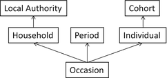

Fig. 10.3
An extension of the multilevel structure of the HAPC, for use with panel data and to incorporate spatial hierarchies. Thus measurement occasions are nested within individuals, which are themselves nested within cohort groups; measurement occasions are also nested into periods and households, the latter of which is additionally nested within local authority districts
Another extension would be to include an interaction between the age and cohort variable in the fixed part of the model. This is particularly useful for panel data, which effectively takes the form of an accelerated longitudinal design (for example see Freitas and Jones 2012). The age-by-cohort interaction allows for the possibility that the life course effect varies by generation – i.e. that there is not a single life course pattern that applies across all cohorts. In our view it is not appropriate to interpret this interaction as a period effect as others have done – for examples see Bell and Jones (2014c); the model still assumes that period effects are absent. The presence of an age-by-cohort interaction term is often thought of as a threat to inference about the life course, that is, a problem that needs to be corrected for (Miyazaki and Raudenbush 2000). However it seems to us that the interaction term can itself be of substantive interest, in understanding how life course trajectories have changed with changing cohort groups. Such an approach is increasingly common in the social medical sciences (Yang 2007; Shaw et al. 2014; Chen et al. 2010; Yang and Lee 2009), and in sociology more generally (McCulloch 2014). However, such designs are usually not combined with the cross-classified structure that characterises the HAPC model.
The model can be further elaborated by adding covariates at any level, or by allowing the effect of variables to vary at certain levels. For example, one could allow the life course (age) effects to vary between individuals, as is regularly done in simpler multilevel life course studies. One could also include control variables of various types, and interact these with the age and cohort variables to test whether the effects of these variables is constant over various dimensions of time.
Stay updated, free articles. Join our Telegram channel

Full access? Get Clinical Tree


