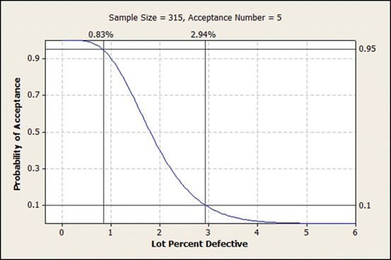
Fig. 20.1
Operating characteristic (OC) curve
Figure 20.1 shows a vertical line drawn at the lot percent defective value of 1.5 %. The value on the vertical axis where the vertical line crosses the OC curve is 0.662=66.2 %. This means that if the true percentage of defective units in the lot is 1.5 %, there is a 66.2 % probability the lot will be accepted. One desires to accept a lot when the percentage of defective units in the lot is acceptably low, and reject the lot when the percentage of defective units in the lot is unacceptably high. Thus, definition of a sampling plan requires definition for both acceptable and unacceptable quality as well as the risks for making incorrect decisions. This process is consistent with the risk based approach advocated in ICH Q9 (ICH 2005).
When deciding whether to accept or reject a lot, there are two types of errors:
1.
Rejecting a good lot (Type 1), and
2.
Accepting a bad lot (Type 2).
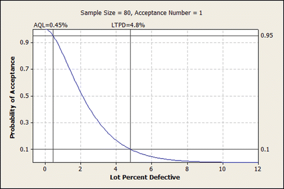
The risk of committing a Type 1 error is referred to as the producer’s risk and is denoted with the Greek letter α. The risk of committing a Type 2 error is called the consumer’s risk and is denoted with the Greek letter β. Definitions for “good” and “bad” are typically defined in terms of the percentage of nonconforming units in the lot. Acceptable quality level (AQL) is the percentage of defective units on the horizontal axis associated with the 95 % probability of acceptance on the vertical axis of the OC curve. The lot tolerance percent defective (LTPD) is the percent defective shown on the horizontal axis associated with the 10 % probability of acceptance (see Fig. 20.2). It is useful to also define AQL and LTPD in terms of the proportions  and
and  .
.
 and
and  .
.
Fig. 20.2
AQL and LTPD on OC curve
The OC curve is based on a realistic compromise between consumer and producer under the recognition that production of perfect product is not realistic. For purposes of this chapter, AQL represents the level of producer quality associated with a probability of acceptance of 95 % and LTPD represents the level of consumer quality associated with a probability of acceptance of 10 %. (Note that LTPD is sometimes represented using other acronyms, most notably as rejectable quality level (RQL)). Using these definitions, Fig. 20.2 shows that the OC curve presented in Fig. 20.1 has an AQL value of 0.45 % and a LTPD value of 4.8 %. (Figures in this chapter were created using Minitab Version 16 Minitab Statistical Software 2015).
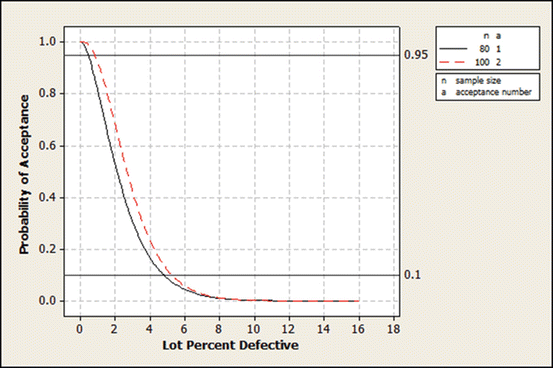
The OC curve changes as the sample design changes. Comparison of the AQL and LTPD values from two OC curves is an appropriate manner for selecting a sampling design. Figure 20.3 shows two sampling plans. The first plan is the same one shown in Fig. 20.1 represented as  . This notation means the lot is accepted if a sample of n = 80 units includes only a = 1 or fewer defective units. Also shown in Fig. 20.3 is the plan
  . For this plan, a sample of n = 100 units is selected, and the lot is accepted if there are a = 2 or fewer defective units. To determine the better sampling plan, one can compare the two OC curves as shown in Fig. 20.3.
 . This notation means the lot is accepted if a sample of n = 80 units includes only a = 1 or fewer defective units. Also shown in Fig. 20.3 is the plan
  . For this plan, a sample of n = 100 units is selected, and the lot is accepted if there are a = 2 or fewer defective units. To determine the better sampling plan, one can compare the two OC curves as shown in Fig. 20.3.
Fig. 20.3
Comparison of two sampling plans
In this situation, at both the 95 % and 10 % probabilities of lot acceptance, the lot percentage defective is lesser for  .
.
 .
.Determination of acceptable values for AQL and LTPD require assessment of a variety of criteria including risks, costs, and consumer requirements. The first step in this process is to classify the severity of the defects that might occur. Typical classifications are Critical, Major, and Minor. Defectives of the same category would generally be expected to have the same values for AQL and LTPD.
20.4 Attribute Sampling
The example introduced in Sect. 20.3 describes an attribute sampling plan. Attribute sampling concerns units that can be classified into one of two groups: defective or non-defective. The summary measure that defines the lot quality is the percentage of units in the lot that are defective. Lesser values of this percentage are associated with greater levels of quality. Calculations used to determine the probabilities shown on the vertical axis of the OC curve are based on either the hypergeometric or the binomial probability distribution. If the sample size is less than 10 % of the total lot size (as occurs in most applications), the binomial distribution is adequate for performing the calculations. The probability of acceptance, P a , shown on the vertical axis of the OC curve is not difficult to calculate. Assuming the binomial model, the probability of accepting a lot for the plan (n, a) when the true lot percentage defective is π is

To demonstrate, the probability of accepting a lot using the plan in Fig. 20.2  when π = 0. 45 % is


(20.1)
 when π = 0. 45 % is
A popular set of sampling plans for attribute sampling which evolved from MIL-STD-105E are contained in ANSI/ASQ Z1.4 (ANSI 2008a). To use the tables in ANSI/ASQ Z1.4 one specifies
1.
Lot size,
2.
AQL,
3.
Inspection level, and
4.
Sampling scheme (single, double, multiple).
The sample size selected is determined based on the lot size through the use of code letters. The desired AQL and code letter then determine the values for n and a. The ANSI/ASQ process is thought to be a generally acceptable practice by most regulatory agencies. However, it is not without its drawbacks. First, strict adherence to the overall ANSI/ASQ Z1.4 sampling system requires switching rules that either increase or decrease the sample size on a given lot based on the historical performance of the output. This requires a sometimes complicated record keeping process that might not be feasible or desirable. Second, when sample size is small relative to the total number of units in a lot, lot size has no impact on the calculations needed to derive the OC curve. Thus, increasing sample size as lot size increases can lead to needless oversampling. Third, these plans consider only AQL in determining a sampling design and in that sense, give the appearance of placing lesser importance on the consumer. For these reasons, many companies prefer to select sampling plans based solely on the OC curve with well-defined and meaningful values for AQL and LTPD.
An example is useful to illustrate this point. USP 2015a recommends an ANSI/ASQ Z1.4 sampling plan for batch release purposes to monitor visible particulates in injections after 100 % inspection during manufacturing. It recommends a single sampling plan using General Inspection Level II for normal inspection with AQL = 0.65 %. Suppose a lot consists of 12,000 units. Using Table 20.1 of ANSI/ASQ Z1.4, the sample size code is letter M. From Table II-A, letter M requires a sample size of 315 units with an acceptable number of defective units equal to five units. This provides the plan  .
.
 .
.Table 20.1
Comparison of sampling designs
π | P(A 1 | π) | ASN |
|---|---|---|
0.20 % | 0.953 | 25.5 |
0.65 % | 0.767 | 39.5 |
2.5 % | 0.284 | 75.7 |
5 % | 0.084 | 90.7 |
The attained value for AQL is 0.83 % and for LTPD is 2.94 % as shown in Table X-M where switching rules are not employed. If switching rules are applied, Chart XV-M reports the realized AQL is 0.781 % and LTPD is 2.12 %. Note that even when switching rules are employed, the attained AQL is greater than the desired value of 0.65 % due to the manner in which tables are constructed.
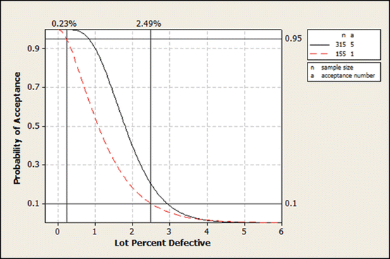
However, stand alone sampling plans that do not require switching rules can be determined directly from an OC curve for any given set of AQL, LTPD, α, and β values. In the present example, USP < 790 > states that “Alternative sampling plans (to ANSI/ASQ Z1.4) with equivalent or better protection are acceptable”. Thus, suppose it is desired to construct an alternative design with AQL no greater than 0.65 % and with LTPD no greater than 2.5 % (assuming α = 0. 05 and β = 0. 10). Figure 20.5 shows one possible design  compared with the OC curve shown in Fig. 20.4. The AQL is 0.23 % and the LTPD is 2.49 % for this alternative design so that USP < 790 > is satisfied. In contrast to the ANSI/ASQ Z1.4 plan, this same sampling design can be used for all lots without the record keeping required to implement the ANSI/ASQ Z1.4 switching rules.
 compared with the OC curve shown in Fig. 20.4. The AQL is 0.23 % and the LTPD is 2.49 % for this alternative design so that USP < 790 > is satisfied. In contrast to the ANSI/ASQ Z1.4 plan, this same sampling design can be used for all lots without the record keeping required to implement the ANSI/ASQ Z1.4 switching rules.
Fig. 20.5
Alternative USP < 790 > Designs
20.5 Variables Sampling
In many situations, quality attributes are measured on a continuous scale and acceptance of a lot is based on the percentage of individual values in a lot that satisfy a numerical specification. The objective is to demonstrate process capability is sufficiently good to provide the desired AQL and LTPD values. To demonstrate, consider the process of accepting a lot of devices that release drug product from a pre-filled syringe. The upper specification limit on the injection time is 15 s. A sample of size n is randomly sampled from the lot and the sample mean is compared to the quantity
 < div class='tao-gold-member'>


Only gold members can continue reading. Log In or Register to continue
Stay updated, free articles. Join our Telegram channel

Full access? Get Clinical Tree


