Fig. 6.1
Formation of magnetoacoustic voltage at tissue interfaces. a Ultrasound wave packet. b Step change in conductivity and density in HMM measurement chamber due to the presence of breast sample. c Conductivity and density gradient at tissue interfaces. d Magnetoacoustic voltage at tissue interfaces
The longitudinal motion of an ultrasound wave in z direction (Fig. 6.1a) will cause the ion to oscillate back and forth in the medium with velocity V 0 . In the presence of constant magnetic field B 0 in y direction, the ion is subjected to the Lorentz force (Wen et al. 1997, 1998; Wen and Bennet 2000).
![$$ {\mathbf{F}} = q[{\mathbf{v}}_{\varvec{z}} \times {\mathbf{B}}_{{\mathbf{0}}} ] $$](/wp-content/uploads/2017/03/A313638_1_En_6_Chapter_Equ1.gif)
(6.1)
The field E 0 and current density J 0 oscillate at the ultrasonic frequency in a direction mutually perpendicular to the ultrasound propagation path and the magnetic field B 0 (x direction). The electric current density is given by (Wen et al. 1997, 1998; Wen and Bennet 2000):
![$$ {\mathbf{J}}_{0} = {\sigma }\left[ {{\mathbf{v}}_{\varvec{z}} \times {\mathbf{B}}_{\mathbf{0}} } \right] $$](/wp-content/uploads/2017/03/A313638_1_En_6_Chapter_Equ3.gif)
(6.3)
Finally, the magnetoacoustic voltage, V, across measurement electrodes a and b due to J 0 can be calculated by the following (Su et al. 2007; Wen 2000; Zeng et al. 2010; Renzhiglova et al. 2010):
![$$ {\mathbf{V}} = \iiint {\left[ {\left( {{\mathbf{v}}_{{\mathbf{z}}} \times {\mathbf{B}}} \right) \cdot {\mathbf{J}}_{\text{ab}} /{\mathbf{I}}} \right] {\text{dV}}} $$](/wp-content/uploads/2017/03/A313638_1_En_6_Chapter_Equ4.gif)
where  is the current density that is induced under the electrodes surface in the breast tissue if a one ampere current, I is applied to the sample through the measurement electrodes (Zeng et al. 2010; Renzhiglova et al. 2010).
(6.4)
is the current density that is induced under the electrodes surface in the breast tissue if a one ampere current, I is applied to the sample through the measurement electrodes (Zeng et al. 2010; Renzhiglova et al. 2010).In addition to that, in ultrasound term, the amplitude of magnetoacoustic voltage in time domain is proportional to (Wen et al. 1998)
![$$ {\text{V}}(t) \propto W\int\limits_{\text{Soundpath initial}}^{\text{Final}} {\frac{\partial }{\partial z}\left[ {\frac{\sigma }{\rho }} \right]\left[ {\mathop \smallint \limits_{0}^{\text{t}} \partial P_{\text{z}} {\text{d}}t} \right]{\text{d}}z} $$](/wp-content/uploads/2017/03/A313638_1_En_6_Chapter_Equ5.gif)
(6.5)
Following the equation of (6.5), gradient σ/ρ is nonzero only at interfaces z1 and z2 (Fig. 6.1c) giving rise to the magnetoacoustic voltage (Fig. 6.1d). The polarity of the two peaks is opposite because the σ/ρ gradients at z1 and z2 are in opposite direction with positive value occur at the transition of low density and conductivity area to high density and conductivity area and vice versa (Wen et al. 1997, 1998; Wen and Bennet 2000; Su et al. 2007; Wen 2000). In a uniform area within the tissue sample, the average ultrasound velocity, v 0 , is zero, and hence, no signal is observed (Wen et al. 1997, 1998; Wen and Bennet 2000).
6.2 Methodology
6.2.1 Experimental Setup
The entire experimental study was conducted in an anechoic chamber with shielding effectiveness of 18 kHz–40 GHz. Electromagnetic shielded environment is preferred to prevent external electromagnetic interference from contaminating the recorded magnetoacoustic voltage and interrupting the sensitive lock-in amplifier readings.
The HMM system consists of a 5077PR Manually Controlled Ultrasound Pulser Receiver unit, Olympus-NDT, Massachusetts, USA. The unit delivered 400 V of negative square wave pulses at the frequency of 10 MHz and PRF of 5 kHz, to 2 units of 0.125-inch standard contact, ceramic ultrasound transducers having the peak frequency of 9.8 MHz. The transducers were used to transmit and receive ultrasound wave in transmission mode setting from the z direction. The pulser receiver unit was also attached to a digital oscilloscope, model TDS 3014B, Tektronix, Oregon, USA, for signal display and storage purposes.
A custom made, 15-cm height, diameter pair magnetized NdFeB permanent magnet is used to produce static magnetic field, with the intensity of 0.25T at the center of its bore. The diameter of the magnet bore is 5 cm, and the direction of magnetic field was set from the y-axis. The overall concept of HMM is shown in Fig. 6.2.
Fig. 6.2
Block diagram of the hybrid magnetoacoustic system. a Side view. b Cross-sectional view
Magnetoacoustic voltage measurements were made from the x direction with respect to the measurement chamber. It was conducted using two units of custom made, ultrasensitive carbon fiber electrodes with 0.1 mm tip diameter. In general, carbon fiber electrode has been used very extensively in the in vivo (Dressman et al. 2002; Yavich and Tilhonen 2000) and in vitro including transdermal (Miller et al. 2011) bioelectrical studies of cells (Chen et al. 2011; de Asis et al. 2010) and tissue of animals (Yavich and Tilhonen 2000; Fabre et al. 1997) and humans (Crespi et al. 1995; Dressman et al. 2002; Shyu et al. 2004). On top of that, its usage in electrophysiological studies and voltammetric/amperometric analysis is perfected by its significantly less noise (Crespi et al. 1995). Furthermore, carbon fiber has a very weak paramagnetic property compared to other conventional electrodes. Due to the property, carbon fiber has been used in combination with fMRI to study the brain stimulation (Shyu et al. 2004). On top of that, carbon fiber electrode is also excellent device with greater sensitivity, selectivity and offers wide range of detectable species since its impedance can be tailored to match the sample under test (Buckshire 2008). In addition to that, many studies reported that carbon fiber electrode has the sensitivity down to 1 nV (TienWang et al. 2006; Han et al. 2004). In this study, the carbon fiber electrodes were connected to a high-frequency lock-in amplifier, model SR844, Stanford Research System, California, USA. The full-scale sensitivity of the amplifier is 100 nVrms (Stanford Research System 1997). Magnetoacoustic voltage measurement was made by touching the tip of the electrodes to the tissue in x direction.
6.2.2 Preparation of Samples
Two types of samples were used in this study. The first sample was a set of tissue mimicking gel with properties that are very close to normal breast tissue. Another sample was a set of animal breast tissues that was harvested from a group of tumor-bearing laboratory mice and its control strain shown in Fig. 6.3. The tissue mimicking gel was used in the early part of this study to understand the basic response of HMM system to linear samples before it was tested to complex samples like real tissues. The same experimental planning was also observed in previous studies (Wen et al. 1997, 1998; Wen and Bennet 2000), in which phantoms were tested to their system before they were tested on real biological tissue.
Fig. 6.3
Transgenic mice strain FVB/N-Tg MMTV-PyVT that carries high-grade invasive breast adenocarcinoma
The tissue mimicking gel was prepared from a mixture of gel powder, sodium chloride (NaCl), and pure water at the right proportion to achieve the desired density and conductivity. Fifteen samples of breast tissue mimicking gel were used in this preliminary study. During the experiment, the samples were cut down to an approximately 1 cm × 1 cm size with 2-mm thickness. Thickness standardization was made using a U-shaped mold with 2-mm opening. Three random samples were chosen for a baseline density and conductivity measurement as shown in Table 6.2.
On the other hand, the use of animal in this study was approved by the National University of Malaysia Animal Ethics Committee. Transgenic mice strains FVB/N-Tg MMTV-PyVT 634 Mul and its control strain FVB/N were obtained from the Jackson Laboratory, USA. For the transgenic mice set, hemizygote male mice were crossed to female non-carrier to produce 50 % offspring carrying the PyVT transgene.
Transgene expression of the mice strain is characterized by the development of mammary adenocarcinoma in both male and female carriers with 100 % penetrance at 40 days of age (The Jackson Laboratory 2010; Bugge et al. 1998). All female carriers developed palpable mammary tumors as early as 5 weeks of age. Male carriers also developed these tumors at later age of onset (The Jackson Laboratory 2010; Guy et al. 1992). Adenocarcinoma that arises in virgin and breeder females as well as males is observed to be multifocal, highly fibrotic and involved the entire mammary fat pad (The Jackson Laboratory 2010; Bugge et al. 1998; Guy et al. 1992). Mice carrying the PyVT transgene also show loss of lactational ability since the first pregnancy (The Jackson Laboratory 2010). Pulmonary metastases are also observed in 94 % of tumor-bearing female mice and 80 % of tumor-bearing male mice (The Jackson Laboratory 2010; Bugge et al. 1998; Guy et al. 1992). The mice female offsprings were palpated every 3 days from 12 weeks of age to identify tumors.
Individual mouse was restrained using a plastic restrainer when the tumor diameter reached 2 cm for the transgenic mice or when it reached 18 weeks of age for normal mice. Anesthesia was performed using the Ketamin/Xylazil/Zoletil cocktail dilution. 0.2 ml of the anesthetic drug was administered intravenously from the mouse tail, and an additional of 2 ml of the drug was delivered intraperitoneally for about 2 h of sleeping time. The fur around the breast area was shaven. The mammary tissue was harvested from the mice while they were sleeping. Mice were then euthanized using drug overdose method. Excised breast specimens were cut down to an approximately 1 cm × 1 cm square shape with thickness of 2 mm immediately after the surgery to maintain the tissue physiological activities. The tissue was carefully trimmed down to the required thickness, and the standardization was made using a custom made U-shaped mold with 2-mm opening. A total of 24 normal and 25 cancerous breast tissue specimens were used in this study. Figures 6.4 and 6.5 show the excised breast tissue specimens. In addition to that, variation in tissue weight for normal and cancerous tissue group is presented in Table 6.1.
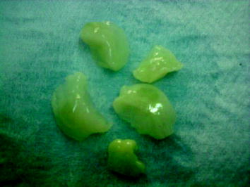
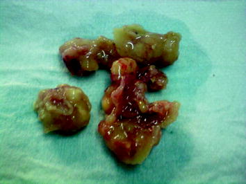
Fig. 6.4
Excised normal breast tissue samples
Fig. 6.5
Excised cancerous breast tissue samples
Table 6.1
Weight variations for normal and cancerous breast tissue samples
No. | Tissue group | Weight variation mean ± std dev (g) |
|---|---|---|
1 | Cancerous tissue | 0.257 ± 0.03 |
2 | Normal tissue | 0.225 ± 0.02 |
The overall process of trimming down after excision took an average time of 6 min, and the samples were immediately immersed in measurement chamber for scanning to maintain their physiological activities. The tissue position in measurement chamber was fixed using a nylon fiber. Previous literature had shown that conductivity measurement is possible to be performed on excised tissue even though the tissue physiological states changes as a function of time following excision or death (Chaudary et al. 1984; Sha et al. 2002). This is because, the termination of blood perfusion after excision leads to the changes in ion distribution between inter- and extracellular spaces (Haemmerich et al. 2002). More specifically, cessation of sodium–potassium pump activity will lead to the depolarization of the cell that results in inflow of sodium and water, which causes cell swelling (Haemmerich et al. 2002; Lambotte 1986). Furthermore, the influx of Ca2+ leads to swelling and rupture of mitochondria that causes cell death.
However, the time taken for those changes to be observed differs according to few factors such as temperature and tissue types (Surowiec et al. 1985; Geddes and Baker 1967). Previous studies showed that conductivity measurement is almost constant in the first hour after the tissue sample had been excised (Chaudary et al. 1984) and measurement is still possible to be made within 4 h (Surowiec et al. 1988). In HMM, the excision of mice breast samples from its domain was done while the mice were sleeping and euthanasia was only performed at the end of the excision process. After excision, the sample was trimmed to the required size and immediately scanned. The time taken from excision to scanning took an average of 6 min and based on the literature presented, it is confirmed that the original conductivity of the breast tissue is retained during the scanning process.
Later, three random samples were chosen for a baseline density and conductivity measurement. Table 6.2 shows the mean baseline conductivity and density value for every group.
Table 6.2
Baseline conductivity and density measurement result
Samples | Conductivity (S/m) | Density (kg/m3) |
|---|---|---|
Normal mice breast | 0.239 | 1,121 |
Cancerous mice breast | 0.547 | 1,319 |
Gel | 0.270 | 1,114 |
6.2.3 Experimental Data Collection
The data collection stage comprises two simultaneous measurements, which are HMM ultrasound measurement and HMM magnetoacoustic voltage measurements.
In ultrasound measurement, specimens were immersed in oil that was located between the ultrasound transmitter and receiver (Mohamad Salim et al. 2010) and its position was fixed using a nylon fiber. The ultrasound transmitter emitted 9.8-MHz ultrasound wave in transmission mode. The transmission mode approach gives some advantages including less complicated data and less noise (Landini and Sarnelli 1986). The distance between the ultrasound transmitter and receiver was set constant to 6 mm. The ultrasound analysis was started and performed at a constant temperature of 21 °C using the insertion loss method described elsewhere previously (Edmonds and Mortensen 1991; Landini and Sarnelli 1986; Mohamad Salim et al. 2010). Sonification was conducted from the z direction. Vegetable oil was used as medium for ultrasound propagation to prevent any leakage current from contaminating the measurement chamber and interfering with the HMM magnetoacoustic voltage output (Su et al. 2007).
A total of 15 gel samples were used in the early part of this study, and the measurement was taken twice for every gel sample. In addition to that, 24 normal and 25 cancerous mice breast tissue samples were also used. Measurement was repeated for five times for every biological sample at any random position on the sample surface.
Additionally, the magnetoacoustic voltage measurement was made by touching the tissue surface from the x direction using the carbon fiber electrodes. The electrodes were attached to the SR844 lock-in amplifier for signal detection and recording. The electrodes tip is the only contact point between the tissue and the detection circuit. The electrodes were manually hold to touch the tissue surface from the x direction with minimal pressure to prevent tissue dislocation from its initial position as well as to prevent measurement instability due to electrodes pressure since conductivity measurement is very sensitive to skin electrodes pressure variations. The input impedance of the lock-in amplifier was set to 1 MΩ, while the time constant was set to 3 ms. However, the experimental reading was updated every 1 s since the amplifier requires a few time constant cycle to stabilize the output reading. The recorded reading of the amplifier was equal to the average voltage of the first and second peak signals. In this study, the lock-in amplifier functions as a high precision voltage reader and a filter that detects signal as low as 100 nV at 9.8 MHz and eliminate other surrounding noises.
The gain of the SR844 lock-in amplifier is calculated by the following equation:

Again, a total of 15 gel samples were used in the early part of this conductivity study, and the measurement was repeated twice for each gel. In addition to that, 24 normal and 25 cancerous breast tissue samples were used and measurement was repeated for five times for every biological tissue sample at any random position on the breast tissue surface at one measurement side (side 1). After the fifth measurement, the tissue orientation was changed to 180° from its initial orientation and measurement was repeated again for five times (side 2).
6.2.4 Experimental Data Analysis
The experimental data analysis stage comprises the analysis of HMM ultrasound output and HMM magnetoacoustic voltage output. In general, the HMM ultrasound output requires further processing in Matlab to find the attenuation scale of the ultrasound wave for every sample via spectral analysis. The objective of processing the HMM ultrasound output is to calculate the power spectral density (PSD) of the signal. It involved the determination of frequency content of a waveform via frequency decomposition. The use of PSD as an estimate of ultrasound attenuation was reported in many studies previously (Edmonds and Mortensen 1991; Mohamad Salim et al. 2010). PSD of the ultrasound signal was plotted in Matlab. The attenuation scale was calculated by subtracting the log mean-squared spectrum of ultrasound signal propagating through the oil without tissue, by the log mean-squared spectrum of ultrasound signal propagating through the oil with tissue, the following equation (Mohamad Salim et al. 2010):
where P s is the mean-squared spectrum of the ultrasound signal propagating in the medium with tissue/gel sample, and P 0 is the mean-squared spectrum of ultrasound signal propagating through medium without sample. Later, the attenuation scale for the gel, normal tissue group, and cancerous tissue group was exported to Microsoft Excel for statistical analysis. The statistical analysis involved the determination of mean and standard deviation for every group.
(6.6)
On the other hand, the recorded magnetoacoustic voltage data was statistically analyzed to find its mean and standard deviation for every sample group (gel, normal tissue, and cancerous tissue).
Both, the ultrasound attenuation value and magnetoacoustic voltage value were fed to an artificial neural network (ANN) for breast cancer classification.
6.2.5 Development of Artificial Neural Network
In this study, an ANN with three inputs was developed for breast cancer classification. A total of 106 ultrasound data and 212 magnetoacoustic voltage data were collected during the experiment. The data were used as an input and target of the ANN. The ANN was trained using the steepest descent with momentum back-propagation algorithm in Matlab environment. The back-propagation algorithm is the most commonly used algorithm in medical computational application as experimented by many studies previously (Ibrahim 2005; Ibrahim et al. 2010). Measurement of ANN performance was made using the mean-squared error (MSE) (Ibrahim 2005; Ibrahim et al. 2010). Training is best when the ANN is capable to achieve the lowest MSE value.
In addition to that, each ANN configuration was tested using the testing group data to obtain the overall prediction accuracy at the end of each training and optimization process (Lammers et al. 2003; Subasi 2005). The aim is to measure the performance of the ANN architecture after each optimization. Using this method, the network was trained using a part of the data and the remainder was assigned as the testing and validation data.
The final process of development is the validation process. In this stage, a set of data that never been used during ANN training was introduced into the ANN for classification. Validation process is very crucial as an assessment of ANN overfitting. Overfitting is usually indicated by low-performance accuracy of ANN to validation data. This explains that the developed ANN is not able to generalize its input and requires new training and optimization process.
Stay updated, free articles. Join our Telegram channel

Full access? Get Clinical Tree


