Some tools of Lean Six Sigma aren’t graphical; they’re simply analytical. Sometimes you want to be able to compare two processes or products and learn something about their quality using statistics alone. Healthcare research often uses these tools to compare the effects of two or more medications or protocols. Six Sigma practitioners can use these tools to compare performance before and after an improvement to verify its effectiveness. This falls under the category of something known as hypothesis testing.
When doing research or clinical trials, these statistical tools help to evaluate the efficacy of various medications or protocols. When using Lean Six Sigma to solve problems, these tools can help to compare the before and after performance to determine whether the results are statistically significant.
HYPOTHESIS TESTING
I’ve come to suspect that hypothesis testing is where statistics got the nickname “sadistics.” I found it confusing because it seems to use negative logic to describe everything. But it’s really not that hard once you understand how it works.
Let’s say that you have two medications or protocols and you want to prove that they are (1) the same (i.e., equal) or (2) different (i.e., not equal) at a certain level of confidence. You might want to compare a control group with a test group to determine whether a medication is effective. Because Lean Six Sigma is obsessed with variation and central tendencies, you might want to prove that the average or variation is the same or different. Hypothesis testing helps you to evaluate these two hypotheses.
The English geneticist who dreamed this up decided that the same or equal result would be called the null hypothesis. Different results are known as the alternate hypothesis. Then, based on the analysis, you want to accept the null hypothesis (i.e., that the two medications or protocols are the same) or reject the null hypothesis (i.e., that the two medications or protocols are different). There are several tools that can help you to do this depending on whether you are most interested in the average or the variation.
HYPOTHESIS TESTING FOR VARIATION
Because variation can affect results, it’s useful to determine whether variation in two or more samples is the same or different. To evaluate variation statistically, use the F-test or Levene’s test.
F-Test for Variation
If you have a single factor measured at two levels (e.g., calcium levels) and you want to know whether they have the same or different variability, use the F-test. An F-test using two samples compares two independent sets of test data. It helps to determine whether the variances are the same or different from each other. Consider the following example.
F-Test Two-Sample Example. If you’re using two different anticoagulants, you might want to know whether the variances for calcium are the same or different.
 Null hypothesis (H0): Variances are the same.
 Alternate hypothesis (Ha): Variances are different.
Now conduct a test and enter the data into Excel (Figure 11.1). Use Excel’s Data Analysis Toolpak under the Tools menu or the QI Macros to conduct the F-test of EDTA versus PPT. The QI Macros will prompt for a significance level (default = 0.05). The F-test will calculate the results (Figure 11.2).
FIGURE 11.1
F-test data.
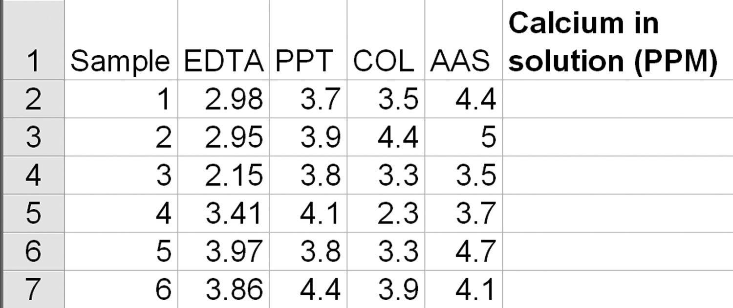
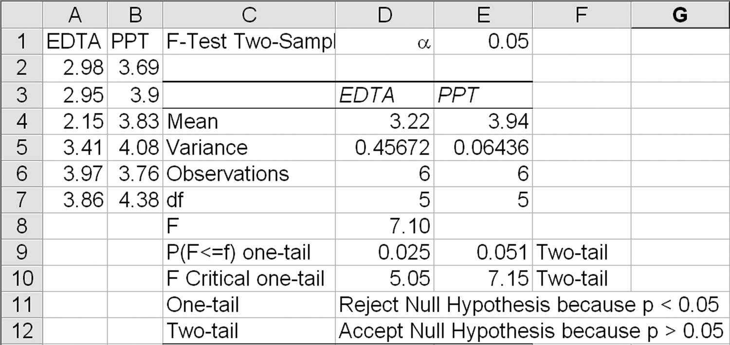
FIGURE 11.2
F-test results.
If you go to www.qimacros.com/trial/hospitalbook, you can download the QI Macros Lean Six Sigma SPC Software 90-day trial. Use the ANOVA tools to access the F-test.
Interpreting the F-Test Results
Hypothesis Test | Compare | Result |
Classical method | Test statistic > critical value (i.e., F > Fcrit) | Reject the null hypothesis |
| Test statistic < critical value (i.e., F < Fcrit) | Accept the null hypothesis |
p-Value method | p < α Reject the null hypothesis | p > α Accept the null hypothesis |
Because F < Fcrit (7.10 < 7.15) and p > α (0.051 > 0.05), we can accept the null hypothesis that the variances are equal (two-tailed) but reject the null hypothesis for one tail.
Levene’s Test for Variation in Non-normal Data
Levene’s test compares two or more independent sets of test data. It helps to determine whether the variances are the same or different from each other. Levene’s test is like the F-test. However, Levene’s test is robust enough for non-normal data and handles more than two columns of data. Consider the following example.
Levene’s Test: Two-Sample Example. Using the F-test example data (see Figure 11.1), conduct a Levene’s test using the QI Macros (Levene’s test is not part of Excel’s Data Analysis Toolpak). The Levene’s test macro will calculate the results (Figure 11.3).
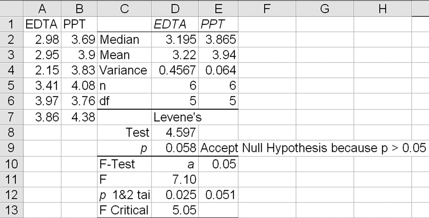
FIGURE 11.3
Levene’s test results.
Interpreting Levene’s Test Results
Hypothesis Test | Compare | Result |
p-Value method | p < α | Reject the null hypothesis |
p > α | Accept the null hypothesis |
Because Levene’s p > α (0.058 > 0.05), we can accept the null hypothesis that the variances are equal.
While an F-test works well on two samples of normal data, it isn’t robust enough to handle non-normal data or more than two samples. (Notice that Levene’s p-value differs from the F-test’s two-tailed value of 0.305, but both result in acceptance of the null hypothesis.)
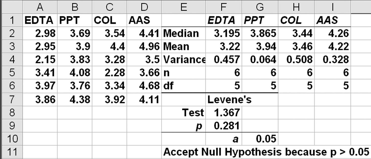
Levene’s Test: Four-Sample Example. Now consider all four anticoagulants (Figure 11.4). Again, p = 0.281, which is greater than 0.05, so we accept the null hypothesis that variances are equal from batch to batch.
FIGURE 11.4
Anticoagulant data.
HYPOTHESIS TESTING FOR MEANS
Because the mean (i.e., average) also affects results, it can be useful to evaluate whether the means of one or more samples are the same or different. There are a number of ways to do this depending on sample size: t-tests, the Tukey test, and ANOVA.
t-Test for Means
t-tests evaluate whether the means of one or two samples are the same or different. There are several types of t-tests:
 t-test: single sample
 t-test: two samples assuming equal variances
 t-test: two samples assuming unequal variances
 t-test: paired two samples for means
t-Test: Single Sample
A t-test using one sample compares test data to a specific value. It helps to determine whether the sample is greater than, less than, or equal to the value. Consider the following example (in QI Macros test data/anova.xls).
Central-Line Bloodstream Infections t-Test Example. Let’s say that you want to know that the improvement to reduce bloodstream infections is statistically below the baseline. So we develop a null hypothesis (H0) that central-line bloodstream infections (CLBSIs) are less than the baseline of 4.85 and the alternate hypothesis (Ha) that CLBSIs are greater than or equal to 4.85:
 H0 < 4.85 infections per 1,000 line days
 Ha ≥ 4.85 infections per 1,000 line days
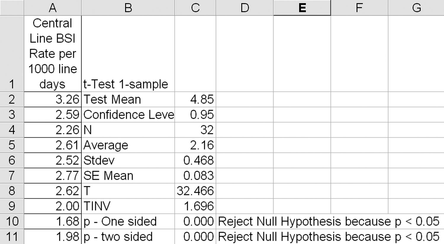
Now take the CLBSI rate after an improvement and enter the data into Excel (column A in Figure 11.5). Then select the data with the mouse, and click on the QI Macros menu to select the one-sample t-test (one-sample t-tests are not available in Excel’s Data Analysis Toolpak). The QI Macros will prompt for a confidence level (default = 0.95, which is the same as a significance of 0.05) and test the mean/average (in this case 4.85). The t-test one-sample macro will calculate the results (columns B and C in Figure 11.5).
FIGURE 11.5
Single-sample t-test data.
Interpreting the t-Test One-Sample Results
If | Then |
Test statistic > critical value (i.e., t > tcrit) | Reject the null hypothesis |
Test statistic < critical value (i.e., t < tcrit) | Accept the null hypothesis |
p < α | Reject the null hypothesis |
p > α | Accept the null hypothesis |
Because the null hypothesis is that CLBSIs are less than 4.85, this is a one-sided test. Therefore, use the one-tail values for your analysis.
Because the t-statistic > tcrit (32.466 > 1.696) and p < α (0.000 < 0.05), we can reject the null hypothesis that CLBSIs are greater than or equal to 4.85. We can say that we are 95 percent confident that CLBSIs are less than 4.85.
Customer-Service t-Test One-Sample Example. Let’s say that you want to know if wait times in an emergency department (ED) are not greater than 3 minutes at a 95 percent confidence level:
 H0 ≤ 3 minutes
 Ha > 3 minutes
Observers collect wait times. This gives us the data we need to test the hypothesis (Figure 11.6).
FIGURE 11.6
Single-sample t-test results.
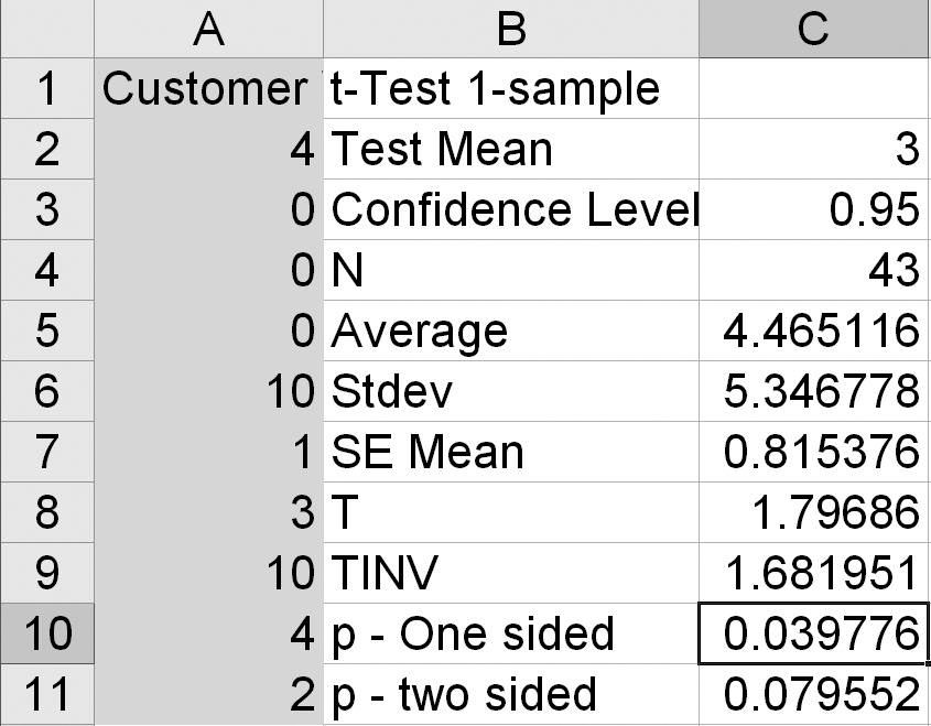
The one-sided p < α [0.039776 < 0.05(1 – 0.95)], so we must reject the null hypothesis that wait times are less than or equal to 3 minutes. We can say that we are 95 percent confident that wait times are greater than 3 minutes.
t-Test: Two Samples Assuming Equal Variances
Using the F-test data from Figure 11.1, you might want to know whether the calcium levels are the same or different between EDTA and PPT.
Define the Null and Alternate Hypotheses
 The null hypothesis H0 is that the mean difference (x1 – x2) = 0 or, in other words, the means are the same.
 The alternative hypothesis Ha is that the mean difference is less than or greater than 0 or, in other words, the means are not the same.
Conduct an F-Test to Determine Whether the Variances Are Equal. Because the two recipes aren’t “paired” or dependent in any way, the first step is to determine whether the variances are equal to determine which t-test to use. Since we’ve already done this, we know that the variances are considered equal for a two-tailed distribution.
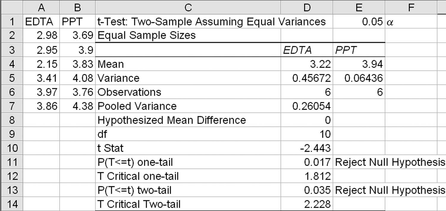
Run the t-Test Assuming Equal Variances. Now select the data with the mouse, and click on the QI Macros menu to select the two-sample t-test (or for Excel’s Data Analysis Toolpak, t-test two samples assuming equal variances). The QI Macros will prompt for a significance level (default = 0.05) and hypothesized differences in the means (default = 0). The t-test two samples assuming equal variances will calculate the results (Figure 11.7).
FIGURE 11.7
Two-sample t-test with equal variances.
Interpreting the t-Test Two-Sample Results
If | Then |
Test statistic > critical value (i.e., t > tcrit) | Reject the null hypothesis |
Test statistic < critical value (i.e., t < tcrit) | Accept the null hypothesis |
p < α | Reject the null hypothesis |
p > α | Accept the null hypothesis |
Because the null hypothesis is that the mean difference (x1 – x2) = 0, this is a two-sided test. Therefore, use the two-tail values for your analysis. Since the t-statistic > tcrit (2.443 > 2.228) and p < α (0.035 < 0.05), we can reject the null hypothesis that the means are the same. Therefore, we can say that the two anticoagulants produce a different calcium level at a 95 percent confidence level.
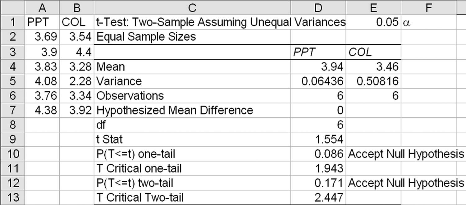
t-Test: Two Samples Assuming Unequal Variances
PPT and COL have different variances, so we could use them to evaluate whether calcium levels are the same or different using these two anticoagulants:
 The null hypothesis H0 is that the mean difference (x1 – x2) = 0 or, in other words, the means are the same.
 The alternative hypothesis Ha is that the mean difference is less than or greater than 0 or, in other words, the means are not the same.
Conduct an F-Test to Determine Whether the Variances Are Equal. Because the two recipes aren’t “paired” in any way, the first step is to determine whether the variances are equal to determine which t-test to use. So select the data (columns A and B in Figure 11.8), and use the QI Macros or the Data Analysis Toolpak to select the F-test.
FIGURE 11.8
Two-sample F-test data.
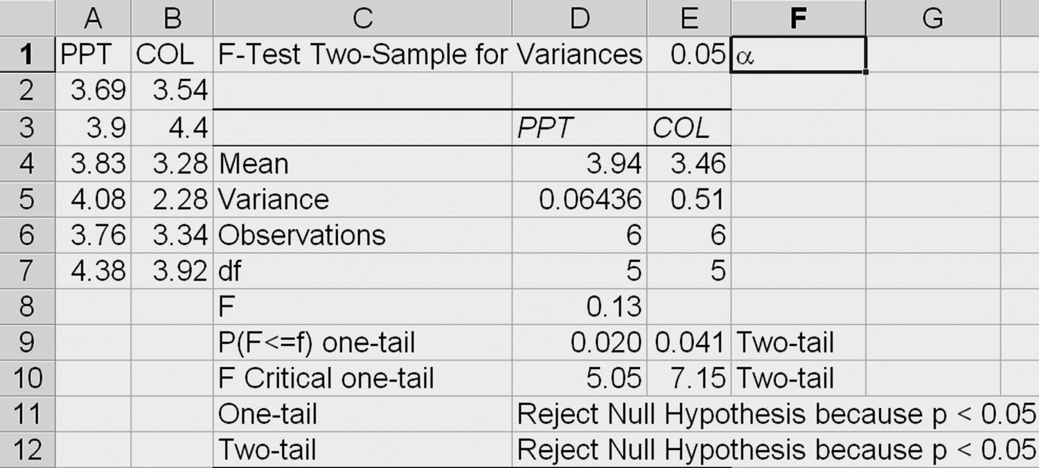
Because p < α (0.0041 < 0.05), we can reject the null hypothesis that the variances are equal. Now we can run the t-test assuming unequal variances.
t-Test Assuming Unequal Variances. Now use the data and the QI Macros or the Data Analysis Toolpak to select the two-sample t-test assuming unequal variances. Enter a significance level (default = 0.05). The two-sample t-test for unequal variances will calculate the results (Figure 11.9).
FIGURE 11.9
Two-sample t-test for unequal variances.
Interpreting the t-Test Assuming Unequal Variances Results
If | Then |
Test statistic > critical value (i.e., t > tcrit) | Reject the null hypothesis |
Test statistic < critical value (i.e., t < tcrit) | Accept the null hypothesis |
p < α | Reject the null hypothesis |
p > α | Accept the null hypothesis |
Because the null hypothesis is that the mean difference (x1 – x2) = 0, this is a two-sided test. Therefore, use the two-tail values for your analysis.
Because the t-statistic < tcrit (1.554 < 1.943) and p > α (0.171 > 0.05), we can accept the null hypothesis that the means are the same. The two anticoagulants produce calcium levels that are equal at a 95 percent confidence level.
t-Test: Paired Two Samples for Means
A paired t-test using two paired samples compares two dependent sets of test data. It helps to determine whether the means (i.e., averages) are different from each other. An example might include test results before and after training (these are paired because the same student produces two results).
The same would be true of weight loss. If a diet claims to cause more than a 10-pound weight loss over a 6-month period, you could design a test using several individuals’ before and after weights. The samples are “paired” by each individual. You might want to know whether the diet truly delivers greater than a 10-pound weight loss. The null hypothesis is weight loss of less than or equal to 10 pounds. The alternate hypothesis is weight loss of greater than 10 pounds.
 H0 ≤ 10 pounds
 Ha > 10 pounds
Stay updated, free articles. Join our Telegram channel

Full access? Get Clinical Tree


