Biostatistics for Healthcare Epidemiology and Infection Control
Biostatistics for Healthcare Epidemiology and Infection Control
Elizabeth A. Tolley
It is common knowledge that investigators face challenges during all phases of planning and implementing research protocols. Clinical and experimental researchers possess the necessary expertise for the medical and scientific aspects of their investigations. Moreover, researchers usually have some knowledge of elementary statistical methods. Some researchers find elementary statistics adequate for their purposes and need only an occasional consultation with a biostatistician. However, recent trends in clinical research, especially in healthcare epidemiology and infection control, indicate increasing complexity that demands a higher level of statistical expertise. These general trends are probably going to continue for the foreseeable future— a situation that may leave a researcher feeling somewhat overwhelmed by all of the tasks to be handled in addition to mastery of subject matter. This chapter discusses the challenges and dilemmas related to statistical issues faced by the researcher during the various phases of planning and implementing a research protocol.
Statistics is the science of collecting, analyzing, interpreting, and presenting data. Descriptive statistical methods involve data reduction and summarizing many observations in a few representative numbers. Biostatistics is the application of statistical methods to biologic, biomedical, or health science problems. Data are numeric observations or measurements that result from a random phenomenon or process (1,2). A random process cannot be controlled, and the data collected can never be reproduced exactly. Data from a random process always contain some natural variation. To identify reasons for observed differences among groups of observations, the researcher must sort out the special causes that lead to systematic variation and separate these from the natural variation that is always present. Consequently, decisions will be uncertain. Before making a decision, the researcher uses statistical inference to objectively evaluate data and quantify the level of uncertainty. In addition, the researcher uses statistical models to represent data in terms of special causes and natural variation; these models aid the researcher in making inferences and decisions based on the data.
The numeric observations are in the form of variables, also called random variables. Certain statistical techniques apply to each type of random variable (1, 2, 3, 4,5,6,7,8,9). Measurement variables may be continuous, if the number of values is very large, or discrete, if only few values (generally <10) are possible. Some measurement variables are actually computed variables, for example, Acute Physiology and Chronic Health Evaluation III (APACHE III) scores. A ranked variable is a measurement variable, the values of which have been placed in ascending or descending order and replaced by the ranks. Attributes must translate into numbers (e.g., frequencies of occurrence or number of infected patients). Attributes are sometimes called categorical variables. If an attribute can be only present or absent, the term dichotomous variable is frequently used.
In today’s clinical studies, even the most focused research protocol can yield enormous amounts of information. The typical clinical setting contains a multitude of measuring devices that can provide exquisitely detailed measurements. Many measurements are collected because of availability rather than need. As a consequence, when a study is concluded, an investigator can be faced with the task of sorting through a huge amount of data. Certain measurements or variables are relevant to and necessary for carrying out the specific objectives of a study. An investigator determines what type of data to collect based primarily on specialized knowledge.
Two concepts have especially important implications for investigators. Accuracy is the closeness of the measure to the true value; lack of accuracy has to do with bias (1, 2, 3,9,10). Before recommending a study or grant for approval and/or funding, most reviewers insist that an investigator show how the results will be unbiased. Thus, the investigator’s responsibility includes demonstrating the experimental validity of the study. Precision is the closeness of repeated measurements to each other (2,3,9). Importantly, precision has no bearing on closeness to the true value. In fact, precision without accuracy can be a problem when an investigator is trying to make statistical inferences.
Most clinical studies involve samples that are chosen from a population, instead of the entire population (2, 3, 4,8,11,12,13). The term population refers to the reference or study population. A random sample is a group chosen from a population such that each member of the sample has a nonzero probability of being chosen, independent of any other member being chosen. A simple random sample is the same as a random sample, except that each member of the population has the same nonzero probability of being chosen. Parameters of the reference population are usually unknown and unknowable. The investigator uses statistics from samples to estimate the parameters of the reference population. Because the sample is smaller than the population, information obtained from the sample is partial, and the investigator uses this information to infer something about the population. Most statistics used in healthcare epidemiology and infection control require the investigator to make the assumptions that (a) the reference population is infinitely large and well defined and (b) the sample behaves like a simple random sample. In practice, the population may not be well defined or infinite. Likewise, the sample may not be random; for clinical studies, samples are often composed of those patients who have been admitted to a particular hospital over a specified period because of certain underlying diagnoses and who have undergone various medical and surgical procedures.
DESCRIPTIVE STATISTICS
In published reports, healthcare epidemiologists summarize patient characteristics with descriptive statistics (1, 2, 3, 4,5,6,7,8,9,11,12,13). Typically, a list of patient characteristics includes measures of central tendency and dispersion for continuous variables.
During the research process, the clinical investigator may start exploratory data analysis by obtaining descriptive statistics of important variables. These descriptive statistics have a variety of other practical uses. For example, a potentially important determinant of disease, such as age, may vary only slightly for those patients included in the study; consequently, the clinical investigator may decide not to consider this variable as a potential risk factor in this study. In addition, the researcher may note which variables have highly skewed distributions and, thus, might yield spurious results during data analysis. Finally, unusually high or low values can be identified and verified, if necessary. The following sections describe descriptive statistics for continuous variables.
Measures of Location or Central Tendency
Location refers to where on an axis a particular group of data is located relative to a norm or another group. Measures of central tendency or central location are used to obtain a number that represents the middle of a group of data.
Mean Mean usually refers to the arithmetic mean or average. The mean is probably the most commonly used measure of location. However, the investigator should be aware that the mean is sensitive to extreme values—both very high and very low values. Other means exist but are used less frequently; the geometric mean is an example. An investigator computes a geometric mean by first taking the logarithm of a group of numbers, computing the mean of the transformed values, and then obtaining the antilog of the mean. Blood pH values are logarithms; however, in practice, after calculating the mean of pH values, no one takes the antilog to obtain the mean hydrogen ion concentration. The Greek letter µ is used to represent the population mean. The sample mean [X with bar above] is an unbiased estimator of µ regardless of the shape of the distribution. If the underlying distribution is normal, then the sample mean is the unbiased estimator with the smallest variance.
Median The median is the 50% point or 50th percentile and, as such, is insensitive to extreme values. If an odd number of observations is ranked from smallest to largest, the median is the middle observation. If an even number of observations is similarly ranked, the median is the average of the n/2 and (n/2) + 1 observations where n is the sample size. For example, if the sample size is 20, after ranking, the median is the average of the 10th and 11th observations. For symmetric distributions, the mean and the median coincide. There is no standard symbol for the median of a population or a sample; however, M can be used for connoting the population parameter or the sample statistic (4).
Mode The mode, or the value with the highest frequency, is a measure of concentration. Distributions may have more than one mode. Distributions with two modes are called bimodal. Trimodal refers to distributions with three modes. For symmetric distributions, the mean, median, and mode have the same value. No standard symbol exists for the mode of a population or a sample.
Measures of Dispersion or Spread
Range The range is the distance between the highest (largest) and the lowest (smallest) value. In healthcare epidemiology, investigators often refer to the interquartile range, which is the distance between the 25th and 75th values. Researchers should report ranges with medians; in this way, information on both location and dispersion can be conveyed to others. For a sample, the range is symbolized by R.
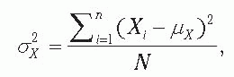
Variance The variance is a measure of dispersion that is often used in calculations. Another name for the variance is the mean square. For populations, the variance is called sigma squared and symbolized with the Greek letter σ2; for samples, the variance is represented by σ2. Because of the availability of inexpensive calculators and spreadsheets with statistical functions, only definitional formulas for the variance of a population and a sample are given, where n is the sample size from a population with N members, and N is much greater than n. For the population, the variance is computed as
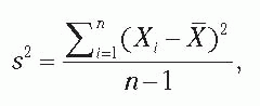
where Xi is the value of the random variable X, measured on each member of the population; i is a unique identifier of each member of the population; m is the population mean for the variable X; Σ signifies summing the squared deviations of the individual values from the mean over all members; and N is the number of members in the population. For the sample, the variance is computed as
where Xi is the value of the random variable X, measured on each observation in the sample; i is a unique identifier of each observation in the sample; [X with bar above] is the sample mean for the variable X; Σ signifies summing the squared deviations over all observations; and n is the number of observations in the sample.
Standard Deviation The standard deviation is the square root of the variance and is sometimes called the root mean square. The standard deviation is a measure of the average distance from the mean. If the standard deviation is small, the observations are crowded near the mean; if the standard deviation is large, there is substantial spread in the data. For populations, the standard deviation is symbolized with the Greek letter σ; for samples, the standard deviation is represented by s. Standard deviations correspond to means. Occasionally, an investigator must approximate the standard deviation of a future sample. The expected range (i.e., the largest value that one expects to record from a future sample minus the smallest value) divided by 4 provides an approximation when no other information is available.
Other Descriptive Measures
Measures of Skewness Measures of skewness and kurtosis may be computed to evaluate how a distribution deviates from a normal distribution. Most clinical investigators do not routinely need these measures. In practice, the investigator may plot the distribution of the data to evaluate the presence of outliers, those observations with values much larger or smaller than the rest of the sample. A distribution that has a few to a moderate number of high values and a mean that is greater than the median is generally referred to as right or positively skewed. Conversely, a distribution that has a few to a moderate number of low values and a mean that is smaller than the median is generally referred to as left or negatively skewed. In summary, the direction in which the tail of the distribution points characterizes the direction of skew.
Kurtosis Kurtosis refers to how flat or peaked the distribution is relative to the normal distribution. If a distribution is flatter than the normal distribution, it is called platykurtotic. On the other hand, if a distribution is more peaked than the normal distribution, it is called leptokurtotic. For kurtotic distributions, the mean and the median coincide, but the standard deviation is either larger or smaller, respectively, than it would have been if the observations were sampled from a normal distribution.
Coefficient of Variation The coefficient of variation allows the researcher to compare two or more standard deviations, because the standard deviation has been standardized by the mean. The population coefficient of variation is (σ/µ)100%, and the sample coefficient of variation is (s/[X with bar above])100%. For most biologic data, the standard deviation increases as the mean increases. Therefore, the coefficient of variation of a particular variable tends to be rather stable over a wide range of values. For experimental studies, the coefficient of variation is an indicator of the reproducibility of the observations. The clinical investigator may use the coefficient of variation to compare variables that may be potential confounders or effect modifiers. For one group of subjects, the spread of different variables may be compared using the coefficient of variation. For two or more groups of subjects, the coefficient of variation may be used to compare the groups with respect to the spread of a particular variable.
PROBABILITY
Many patient characteristics are dichotomous attributes, which are either present or absent, such as fever. Some characteristics have the form of categorical variables with only a few possible states. For example, the investigator may categorize patients according to the presence of a rapidly fatal disease, an ultimately fatal disease, or a nonfatal disease. In some statistical texts, authors apply the term discrete variable to a characteristic or attribute with two or more states. In published reports, healthcare epidemiologists summarize these types of patient characteristics by indicating the proportion of the total group with each characteristic of interest.
During the research process, the clinical investigator often begins exploratory data analysis by considering the relationships between pairs of categorical variables. The following sections contain important rules and definitions that the clinical investigator must master before undertaking a complex study. Dichotomous variables are emphasized, because many clinically important risk factors are dichotomous variables.
Definitions and Rules
Many problems in healthcare epidemiology and infection control involve analysis of frequencies for various attributes (e.g., numbers of patients with and without infections). When only two outcomes are possible, the variable is called a dichotomous variable. For this example, a patient either has an infection or does not and cannot be characterized as being in both states simultaneously. Thus, having an infection is a dichotomous variable that represents mutually exclusive states. The infected state is represented by I and the noninfected state by ł (i.e., I stricken through with a line connoting “not”). The probability that an infection is present is represented by p; the probability that an infection is not present is represented by (1-p). Some authors of statistics texts represent (1-p) as q. Mathematically, we express the probability that a patient has an infection by the expression, Pr(I) =p. Because the states are mutually exclusive and only these two states can occur, p and q, or (1-p), sum to 1.0.
Probability can be expressed as a fraction with a numerator and denominator, a decimal fraction or proportion, or a percentage. In this chapter, probability is always a proportion. Probabilities can have any value between 0 and 1.0, inclusive. For dichotomous variables, a probability of 0 implies that an event (i.e., one of the two possible states) cannot occur; a probability of 1.0 implies that the event will always occur.
Researchers in healthcare epidemiology need a basic understanding of some concepts related to probability. After mastering a few easily understood concepts (i.e., three rules and six definitions), the researcher can achieve a deeper understanding of how and when important statistics, such as risk ratio (RR), are used.
Unconditional or Total Probability In healthcare epidemiology and infection control, researchers must assess total or unconditional probabilities (1, 2, 3, 4,5,8,12,13). The definition of a total probability is illustrated in the following example. The probability that a patient chosen at random has an infection may be calculated as the relative frequency of patients with infections: the numerator is the number of patients with at least one infection, the denominator is the total number of patients in the study. If 15 of 45 patients in the medical intensive care unit (ICU) have at least one infection, the empirical probability of being infected is .33. This probability may be symbolized as Pr(I) = p =.33. Thus, the total probability of an event occurring is the number of times the event occurs divided by the number of times that it could have occurred.
Empirical Versus Theoretical Probabilities A clinical investigator obtains empirical probabilities from the sample of patients in the particular study. A better method for estimating the true or theoretical probability of a future patient, π, having at least one infection would involve enumerating all infections in all the patients over a long period. The investigator could continue to expand the sample size by including other units and other hospitals and so on. Finally, after the investigator had gathered a very large group of patients from many locations, the empirical probability would approach the theoretical probability of an average hospitalized patient having an infection. Thus, the theoretical probability of infected patients is the relative frequency for cases of infection over an infinitely large sample. During an investigation of a possible outbreak of disease, infection control officers compare empirical probabilities, p, with theoretical probabilities, π.
Conditional Probability In healthcare epidemiology, researchers are also interested in conditional probabilities (1,3,4,5,8,12,13). An example of a conditional probability is the probability of pneumonia, given that the patient has been intubated. The condition states the circumstances restricting the type of patients of interest to the researcher. A researcher obtains a conditional probability of healthcare-associated pneumonia given intubation by (a) enumerating the number of patients with the two characteristics (i.e., intubated patients with pneumonia) and (b) dividing by the number of patients who are intubated (i.e., those at risk for ventilator-associated pneumonia). In this example, the conditional probability of having pneumonia given that the patient is intubated may be symbolized by Pr(P|V), where | indicates given, P symbolizes a patient with pneumonia, and V symbolizes a patient who is intubated or on a ventilator. Therefore, if 25 patients are ventilated and have healthcare-associated pneumonia and 100 patients are ventilated, Pr(P|V) = 25/100 = .25.
Joint Probability and the Product Rule The first rule of probability considered in this chapter is the product rule (1,3,4,5,8,12,13). The product rule states that for any two events A and B, the joint probability of events A and B occurring together is equal to the product of the conditional probability of A given B times the total probability of B. In this example, the probability of being intubated and having pneumonia is obtained by multiplying the conditional probability of having pneumonia given that the patient is intubated by the probability of the patient being intubated. In the ICU, the joint probability that a patient selected at random will be both intubated and have pneumonia may be symbolized mathematically by Pr(P and V), where P indicates a patient with pneumonia and V indicates a patient who is intubated or on a ventilator. In this example, if Pr(V) = .40 (i.e., 40% of the patients in the study are ventilated) and Pr(P|V) = .25 (i.e., 25% of the intubated patients have pneumonia), then Pr(P and V) = Pr(P|V) × Pr(V) =.25 × .40 = .10. Thus, 10% of the patients in the study have both characteristics.
Independent and Dependent Events Often the healthcare epidemiologist will want to know if there is an association between two events (1,3,4,5,8,12). No causal relationship can be identified without substantially more evidence than that provided by one investigation. In this example, the researcher might be looking for an association between a patient being intubated and development of healthcare-associated pneumonia. Therefore, the epidemiologist wishes to know if the ventilated patients in the study are more likely to develop pneumonia than expected based on the theoretical probability of healthcare-associated pneumonia in the particular ICU. In making this decision, the epidemiologist determines the probability of an average patient developing pneumonia and being intubated under the assumption that these two events are independent (i.e., they have no association). Under independence, Pr(P and V) = Pr(P) × Pr(V). If 20% of the patients in the study have pneumonia, then Pr(P) = .20. Thus, if there is no association between being on the ventilator and developing pneumonia, Pr(P and V) = .20 × .40 = .08. This result implies that one would expect 8% of patients to be ventilated and to develop pneumonia if the assumption of independence is correct for this situation. Based on previous computations, the investigator knows that, in this study, 10% of the patients actually have both characteristics. Because the empirical probability is not the same as the theoretical probability, the conclusion is that there is evidence of an association between intubation and pneumonia. Determining whether this association is evidence of a special cause or merely a reflection of natural variability requires the researcher to use inferential statistics. Inferential methods appropriate for this example are presented in other sections.
In this example, the researcher could have reached the same conclusion by comparing total and conditional probabilities. Under independence, the probabilities are equal; therefore, Pr(P|V) = Pr(P). For the healthcare epidemiologist, this statement implies that with respect to a patient developing pneumonia, the ventilator is neither a risk factor nor a protective factor; therefore, patients on the ventilator have the same risk of developing pneumonia as any other patient in the study. For this example, Pr(P |V) is .25, a value that is greater than Pr(P) = .20. When these two probabilities are unequal, there is evidence of an association between the two variables of interest.
Addition or Total Probability Rule The second rule is called the addition or total probability rule (1,3,4,5,8,13). This rule states that for any two events A and B, the total probability of A equals the sum of the joint probability of A and B plus the joint probability of A and not B: Pr(A) = Pr (A and B) + Pr(A and not B). For convenience, these probabilities are often displayed in a 2 × 2 table. Accordingly, the term marginal probability is used interchangeably with total probability.
Before continuing the discussion of probability, the layout of a 2 × 2 table is considered. Statistically, no restriction exists that stipulates placement of exposure and disease on a particular margin or the order in which presence and absence are given on a particular margin. However, the interpretability of some measures of association, which specifically apply to epidemiology, depends on a particular arrangement. When an investigator devises a 2 × 2 table, the proportion of patients with the two attributes and those without the two attributes should be placed on the main diagonal (i.e., cells 1 and 4 of the following table). Epidemiologists have developed other conventions, the use of which has helped to standardize presentation of data. Furthermore, some statistical software products have specific requirements for placement of attributes.
Exposed to Ventilator
Not Exposed to Ventilator
Total or Marginal Probability of Disease
Pneumonia present
p1
p2
p1 +p2
Pneumonia absent
p3
p4
p3 + p4
Total probability of exposure
p1 + p3
p2 + p4
In the previous table, p1, p2, p3, and p4 are joint probabilities. For this example, p1 is the joint probability of a patient having both exposure to the ventilator and pneumonia. Marginal probability of pneumonia can be calculated as the sum of the joint probabilities. In this example, the probability of having pneumonia, Pr(P), equals the sum of the joint probabilities, Pr(P and V) and Pr(P and ) (i.e., p1 + p2). The other total probabilities, Pr(), Pr(V), and Pr(), can be calculated by using the addition rule and are displayed in the following table.
Exposed to Ventilator
Not exposed to Ventilator
Total or Marginal Probability of Disease
Pneumonia present
Pr(P and V)
Pr(P and )
Pr(P)
Pneumonia absent
Pr( and V)
Pr( and )
Pr()
Total probability of exposure
Pr(V)
Pr()
1.0
Alternatively, using the definition of joint probability, the healthcare epidemiologist can replace the joint probabilities p1 and p2 with the product of the conditional probability of disease multiplied by the respective probability of exposure. The same can be done with p3 and p4. Frequently, the healthcare epidemiologist uses this approach when the research question involves identifying risk factors. Typically, the healthcare epidemiologist asks that question before designing a prospective study.
Exposed to Ventilator
Not Exposed to Ventilator
Total or Marginal Probability of Disease
Pneumonia present
Pr(V) × Pr(P|V)
Pr() × Pr(P|)
Pr(P)
Pneumonia absent
Pr(V) × Pr(|V)
Pr() × Pr(|)
Pr()
Probability of exposure
Pr(V)
Pr()
1.0
Finally, a healthcare epidemiologist may wish to study a particular exposure and describe the relationship of that exposure to the presence of a particular disease. In this example, the investigator would be interested in the probability of exposure to the ventilator given that a patient has pneumonia. Usually, the healthcare epidemiologist asks this question before designing a retrospective study, often a case-control study.
Exposed to Ventilator
Not Exposed to Ventilator
Total Probability of Disease
Pneumonia present
Pr(P) × Pr(V|P)
Pr(P) × Pr(|P)
Pr(P)
Pneumonia absent
Pr() × Pr(V|)
Pr() ×Pr(|)
Pr(P)
Probability of exposure
Pr(V)
Pr()
1.0
In the healthcare setting, patients are exposed simultaneously to several risk factors. By considering each exposure separately, the healthcare epidemiologist can use this approach to identify the most likely route of exposure given a particular disease.
In summary, when the healthcare epidemiologist investigates the relationship between two dichotomous events (e.g., exposure and disease), the 2 × 2 table provides a useful and flexible way of displaying the relative frequencies at which the four possible combinations of exposure and disease occur in the sample. Depending on the specific research question, the investigator chooses the most meaningful way to express p1, p2, p3, and p4.
Applications Relevant to Epidemiology
Epidemiologists measure morbidity in terms of prevalence and incidence. Several applications of probability to epidemiology require the investigator to recognize the distinction between these two measures. Prevalence is the proportion of individuals who have the disease. Stated another way, prevalence is the proportion of individuals who have the disease out of all individuals in the population (i.e., those who are at risk for the disease). Prevalence can be defined as the probability that an individual has the disease regardless of the time elapsed since diagnosis. In contrast, incidence is the rate at which new cases occur among individuals who were disease free. Incidence is the number of new cases that have occurred over a specified time divided by the number of individuals who were disease free (i.e., at risk for the disease) at the beginning of the period. Therefore, incidence can be defined as the probability that a disease-free individual will develop the disease over a specified period.
Relative Risk or Risk Ratio RR is the ratio of the incidence of a disease among exposed persons to the incidence of a disease among unexposed persons (1,3,5,8,12, 13, 14, 15,16,17,18,19,20,21,22). Often, epidemiologists use the term risk ratio interchangeably with relative risk. Values for RR are positive and range theoretically from zero to infinity; however, in practice, the denominator probability (i.e., incidence of disease in the unexposed) determines the upper limit for RR. For example, if the incidence of disease in the unexposed is 0.4, then the upper limit for RR is 2.5. This restriction limits the direct comparability of RRs across locations or studies.
If the probability of disease is equally likely for those exposed and those not exposed, the RR equals 1.0. Whenever the RR equals 1.0, exposure and disease are independent. If the probability of disease is higher for those exposed than for those not exposed, RR is >1.0 and exposure is a risk factor. If the probability of disease is lower for those exposed than for those not exposed, RR is less than 1.0 and exposure is a protective factor. As the RR of disease increases or decreases from 1.0, there is evidence that the two events, exposure and disease, are associated or dependent. Using the information in a tabled display, the infection control officer can obtain two conditional probabilities: Pr(P|V) = .25 and Pr(P|) = .167. Thus, the RR is 1.497. In this situation, the officer would conclude that according to these data, a patient on a ventilator is about 1.5 times as likely to develop pneumonia as a patient who is not on a ventilator.
Odds Ratio When incidence is not known, RR cannot be obtained. However, the RR can be approximated by the odds ratio (OR) (1,5,8,12, 13, 14,15,16,17,19,20,21,22). If the proportion of diseased persons (i.e., prevalence) is small (i.e., <0.1), then the OR is usually a reasonably good approximator of the RR. Therefore, the investigator is responsible for carefully evaluating the OR as an approximator of the RR. In making this evaluation, the investigator must consider whether the disease is chronic or acute. Approximation of the RR is biased when only prevalent cases are used in the analysis. When the duration is short (because of either rapid fatality or cure), the numbers of incident and prevalent cases are very nearly the same; very little bias in approximating RR based on prevalent cases is likely. However, when duration is long, bias can be a problem. For example, when serum cholesterol is used to predict death from heart disease, the OR from prevalent cases is lower than the RR from incident cases. This downward bias occurs, because the individuals with the highest cholesterol values are more likely to have a high fatality rate and thereby to escape detection as prevalent cases. In addition, the investigator should be aware that for a particular sample, the OR will have a more extreme value compared with the RR. If the estimates of the OR and RR based on the sample are >1.0, the estimated OR will be larger than the estimated RR. Conversely, if the estimates of the OR and RR based on the sample are <1.0, the estimated OR will have a value smaller than the estimated RR.
Both RRs and ORs are very useful statistics and have many applications for observational and quasi-experimental studies. Although the clinical investigator often makes the same inferences from an OR as from an RR, these statistics are not interchangeable. Therefore, investigators should be very strict in stipulating whether an estimate is an RR or an approximation based on an OR. Furthermore, it is incumbent on the investigator to demonstrate the validity of any implicit assumption that the approximation based on an OR is a good approximation of RR. Failure to do so can have dangerous consequences involving misinterpretation of published reports and erroneous clinical decisions about patient care.
From the first table, the RR may be computed as a ratio with p1/(p1 + p3) in the numerator and p2/(p2 + p4) in the denominator. If the number of patients with pneumonia is small, p1 will contribute very little to the quantity (p1 + p3); likewise, p2 will contribute very little to the quantity (p2 + p4). The OR equals a ratio with p1/p3 in the numerator and p2/p4 in the denominator. Statistically, the OR can always be used to approximate the RR. As p1 and p2 become smaller, the OR may become a better approximator of the RR. Like RR, the OR ranges theoretically from zero to infinity. However, the OR has a property that can make it a more useful statistic than the RR. The OR is independent of the denominator probability (i.e., an OR of 2.0 has the same meaning regardless of the population or sample on which it was based). The OR is considered the odds of having the disease with the factor present relative to the odds of having the disease with the factor absent. The OR may be calculated from a 2 × 2 table by calculating the ratio of cross-products (multiplying diagonally): OR = (p1p4)/(p2p3).
Sensitivity, Specificity, and Predictive Value The healthcare epidemiologist can use joint, conditional, and total probabilities for quantifying commonly used laboratory tests (5,8,12, 13, 14,15,16,17,18,19,20,21,22,23,24,25,26). The total or marginal probability of disease may be represented as Pr(D); this probability is an estimate of disease state prevalence in a population. Prevalence can be thought of as the underlying probability of disease state in a particular population. Likewise, Pr() can be thought of as the underlying probability of not having the disease state; it is not necessarily the probability of wellness or health.
In terms of conditional probability, the probability of a positive test result given that a patient has the disease—that is, Pr(T|D)—refers to test sensitivity. Similarly, the probability of a negative test result given that a patient does not have the disease—that is, Pr(|)—refers to test specificity. The sensitivity and specificity of a test are independent of prevalence.
The healthcare epidemiologist can display the various possible combinations of disease states and test results in a 2 × 2 table.
Positive Test Result
Negative Test Result
Marginal Probability
Disease present
Pr(D) × Pr(T|D)
Pr(D) × Pr(|D)
Pr(D)
Disease absent
Pr() × Pr(T|)
Pr() × Pr(|)
Pr()
Marginal probability
Pr(T)
Pr()
1.0
In contrast, the predictive values of a positive test result (PV+) and a negative test result (PV-) depend on prevalence. In terms of conditional probability, the probability of a patient having the disease given that the test result is positive —that is, Pr(D|T)—refers to positive predictive value of the test (PV+). Similarly, the probability of a patient not having the disease given that the test result is negative— that is, Pr (|)—refers to negative predictive value of the test (PV−).
Positive Test Result
Negative Test Result
Marginal Probability
Disease present
Pr(T) × Pr(D|T)
Pr() × Pr(D|)
Pr(D)
Disease absent
Pr(T) × Pr(|T)
Pr() × Pr(|)
Pr()
Marginal probability
Pr(T)
Pr()
1.0
Alternatively, the healthcare epidemiologist may interpret this table in terms of joint probabilities. From this perspective, the epidemiologist considers the probability of an average (or random) patient having a test result that is considered true positive (TP), true negative (TN), false positive (FP), or false negative (FN). Specifically, the probability of a TP test result is a joint probability—that is, Pr(T and D). The other three outcomes may be expressed similarly as joint probabilities. The probability of obtaining a TN result is the joint probability of testing negative and not having the disease. The probability of obtaining an FP result is the probability that a patient selected at random will test positive but not have the disease. Finally, the probability of obtaining an FN result is the probability of a patient selected at random testing negative but having the disease. In practice, these probabilities are often expressed as percentages. These probabilities may be displayed as follows.
Test Results
Positive
Negative
Total Probability
Disease present
Pr(TP) = Pr(T and D)
Pr(FN) = Pr( and D)
Pr(D)
Disease absent
Pr(FP) = Pr(T and )
Pr(TN) = Pr( and )
Pr()
Total probability
Pr(T)
Pr()
1.0
Prevalence is the sum of the probability of a TP result and the probability of an FN result. Similarly, the probability of testing positive is the sum of the probability of a TP result and the probability of an FP result. The other two marginal probabilities can be obtained in the same way.
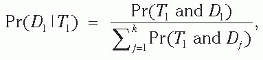
Bayes’ Theorem In more complex situations, the healthcare epidemiologist encounters more than two possible clinical signs or symptoms (symbolized as Ti, where i indicates the alternative clinical signs and symptoms) and more than two possible disease states (symbolized as Dj, where j indicates the alternative disease states). The 2 × 2 tables can be expanded into i columns and j rows, representing clinical findings and disease states, respectively. Bayes’ theorem or rule allows the healthcare epidemiologist to obtain the conditional probability of a particular disease given a particular clinical finding (1,3,5,8,12,15,16,18,25). Bayes’ theorem or rule states that the conditional probability of D1 given T1 equals the joint probability of T1 and D1 divided by the sum of the joint probabilities of T1 and each Dj:
where (a) Pr(Dj) represents the known probabilities of disease states in a specified population and the sum of all Pr(Dj) values equals 1.0 and (b) the various Dj values are mutually exclusive (i.e., a patient cannot have more than one disease). When healthcare epidemiologists need to choose the most likely explanation for their clinical findings, they often use Bayes’ rule to assess the conditional probabilities of several disease states in light of their particular clinical findings. In published literature, epidemiologists may use conditional probabilities to discuss the merits of several alternative explanations. Clinicians may use Bayes’ rule to evaluate a number of diagnostic possibilities. They realize that although no test is absolutely accurate, positive test results do tend to increase the probability that a particular disease is present. The conditional probability of disease given certain clinical findings provides a number that quantifies the amount of confidence that can be placed in stating that a particular disease is present. Differential diagnosis, decision theory, and decision making involve applications of Bayes’ rule.
HYPOTHESIS TESTING
Hypothesis testing does have a place in analysis of data related to healthcare epidemiology and infection control. One-sample tests can be used to determine whether the sample is different from the reference population. Clinical investigators often use two-sample tests during exploratory data analysis to identify potentially important risk factors. The following sections address general definitions and rules for hypothesis testing for one- and two-sample tests for categorical and continuous variables using parametric and nonparametric methods.
Definitions and Rules
The hypothesis is always formulated about parameters. H0 designates the null hypothesis and H1 the alternative hypothesis. Based on sample statistics, the healthcare epidemiologist chooses which is the true situation. For a one-sample hypothesis test, the reasons for this choice are based on how likely it is that these data could have been obtained from a specified reference population. Similarly, for a two-sample hypothesis test, the reasons are based on how likely it is that the difference between the two groups obtained from these data could have occurred given that H0 is true. In making this decision, the epidemiologist may make errors. Naturally, minimizing the probability of making an erroneous decision is a paramount concern of the epidemiologist, even though the truth remains unknown and unknowable. The decisions that an epidemiologist can make relative to the truth (1,2,4,5,8,10,25) are displayed in the following 2 × 2 table.
Unknown But True State of Nature
Decision in Favor of
H0 True
H1 True
H0
Correct
Type II error
H1
Type I error
Correct
Traditionally, scientific investigators have agreed on the principle of keeping the probability of a type I error as small as possible. Pr(type I error) is the conditional probability of rejecting H0 when H0 is correct. Stated another way, Pr(type I error) is the probability of rejecting H0 given that H0 is correct. Statisticians have symbolized Pr(type I error) as α. Another commonly used name for Pr(type I error) is the significance level. The interpretation of a p value is consistent with the definition of the probability of a type I error; a p value gives the probability of finding a result that is at least this extreme, assuming that the H0 is true. Stated another way, the p value qualifies the rejection of H0 with a level of significance. An investigator rejects H0 when the p value is less than α. The p value tells others the statistical significance of the results. Statistical significance has absolutely nothing to do with the scientific or clinical importance of findings.
Another type of error is possible—type II error. Pr(type II error) is the conditional probability of not rejecting the H0 when H1 is true. Stated differently, Pr(type II error) is the probability of deciding in favor of H0 given that H1 is correct. Statisticians have symbolized Pr(type II error) as β. In practice, statisticians are more concerned with power, symbolized as 1-β. Power is the probability of discriminating between H0 and H1, (a) given a specified sample size, a stipulated difference between the values of the parameter under H0 and H1, and a particular α; and (b) assuming H1 is true. Thus, power is the probability of rejecting H0 when H1 is true. Power depends on α, H0 and H1, and sample size. As α decreases, β increases. As the difference between H0 and H1 decreases, power decreases. As sample size increases, power increases—power is very dependent on sample size. Investigators want power to be as large as practically possible, because power represents the probability of correctly rejecting H0. Typical values for power are 0.80, 0.90, 0.95, and 0.99. Before recommending a clinical trial for approval and/or funding, most reviewers insist that the investigator show that the likelihood of getting conclusive results (i.e., statistical power) is high. In unplanned clinical studies, power may be as low as 0.20 or occasionally even lower. Sometimes, epidemiologists compute power after a study has been completed. Under these circumstances, power is the probability of discriminating between H0 and H1, given the findings of the study.
Hypothesis Tests for Categorical Data
A random variable is a numeric quantity that has different values, depending on natural variability. A discrete or categorical random variable is a variable for which there exists a discrete set of values, each having a nonzero probability. Many data from biologic and medical investigations have a common underlying structure.
Cumulative incidence and prevalence of a disease are distributed binomially (1,8,12). Variables that follow a binomial frequency distribution are characterized by the following criteria: (a) a sample is taken of n independent trials, (b) each trial may have two possible outcomes (e.g., success/failure, present/absent, alive/dead), and (c) the probabilities for the outcomes are a constant p for success and (1-p) =q for each failure for every trial. Usually a healthcare epidemiologist is not concerned with the order in which the failures occurred; instead the epidemiologist is interested in the number of failures and the probability that a number as extreme or more extreme occurred given that H0 is true.
Generally, an incidence density variable follows a binomial distribution. For variables such as incidence density, the Poisson distribution is often an accurate approximation of the binomial distribution. The Poisson distribution is a discrete frequency distribution of the number of occurrences of rare events (1,8,12). For the Poisson distribution, the theoretical number of trials is infinite and the number of possible events is also very large. Incidence density studies often involve one or more cohorts of disease-free individuals. A failure is defined as the occurrence of the disease of interest in a previously disease-free individual. The probability of k events (i.e., failures) occurring in a period of time T is defined for a Poisson random variable. Thus, the Poisson distribution depends on two parameters: the length of the interval, T, and the underlying λ, which represents the expected number of events per unit of time. Time may also be defined as a combination of time and level of exposure (e.g., pack-years of smoking or patient-days in the ICU). The mean and the variance of a Poisson distribution are the same. For variables that follow a binomial distribution, when n is large and p is small, the mean and variance will be similar; thus, the Poisson may be used as an approximation of the binomial.
The following two sections describe statistical methods for one- and two-sample tests on binomial proportions or rates (1,3,4,5,6,7,8,15,18,25,27). Throughout these sections, unless otherwise stated, the significance level is .05; power is 0.80; and all tests are two-sided. In power and sample size formulas, a z-score for the 97.5th percentile is used for a two-sided test with a significance level of .05: z0.975 is 1.96. When power of 0.80 is used to determine sample size, a z-score for the 80th percentile is used: z0.80 is 0.842.
These sections, describing one- and two-sample tests for binomial proportions or rates, are not designed as casual reading material; instead, they provide a concise reference of commonly used statistical methods. The only formulas included are those for the test statistics. Most clinical investigators use statistical packages for obtaining sample size estimates or power calculations. For appropriate formulas, the reader is referred to various biostatistical textbooks, for example, Rosner (8) or Sokal and Rohlf (2). For a binomial probability, π refers to the population parameter and p refers to the sample statistic, which approximates the parameter. Each section follows the same format, which is outlined in the following.
Step 1. Set up H0 and H1.
The investigator uses the research question to form H0 and H1. Generally, H1 reflects the result that the investigator expects to find (i.e., that there is a special cause that differentiates the study group from the norm). For a onesample hypothesis test, H0 states that the proportion of events or rate of occurrence (π) in the study group is the same as some specified or norm value, π0. The investigator obtains this value, π0, from some source other than the current study. Typically, the investigator obtains π0 from theoretically derived values or uses nationally or locally compiled values. In the one-sample situation, H1 states that the proportion of events or rate of occurrence (π) in the group being studied differs from the specified value, π0. The investigator estimates π from a sample as p. If the estimated value is sufficiently close to the specified value, π0, the investigator decides in favor of H0 (i.e., that the data are consistent with H0 being true). If the data fail to support H0, the conclusion is that the data are not consistent with H0 being true; therefore, the investigator rejects the H0, concluding that the rate or proportion must be some other value (i.e., higher or lower than π0).
For a two-sample hypothesis test, H0 states that the proportion of events or rate of occurrence (π1) from the first group is the same as that (π2) from the second group. For a clinical trial, the groups might reflect those receiving and not receiving the treatment. For an observational study, the groups might reflect those subjects with and without the attribute of interest. Interpretations of failing to reject and rejecting H0 are similar to those described for the one-sample situation.
Step 2. Choose α, power, and the difference between π and π0 (or π1 and π2) that is clinically meaningful. Another term for the difference between π and π0 (or π1 and π2) is effect size. Frequently, investigators overlook this step. For example, the healthcare epidemiologist may not have the opportunity to conduct a formal power analysis before data collection begins. However, whenever the effect size estimated from the sample is clinically meaningful but the results are consistent with H0, the investigator should determine power retrospectively. This analysis allows the investigator to determine how much larger the sample would have to be to reject H0, given the results of the study. Even when statistical significance is achieved, a retrospective power analysis can indicate how cautiously the results should be interpreted.
Step 3. Using an available computer package, determine sample size, n. Sample size is extremely sensitive to the effect size chosen by the investigator.
Step 4. Obtain data.
Step 5. Compute test statistic in terms of parameters under H0. Obtain the p value associated with the test statistic, assuming H0 is correct. The interpretation of the p value is valid only in terms of H0 and H1. By choosing to make a hypothesis test, the investigator restates the research question and must decide between H0 and H1 based on how consistent or inconsistent the data are with H0. The term consistent connotes having sufficient empirical support for the investigator to decide that the unknown true state of nature is likely to be H0 instead of H1. Conversely, the term inconsistent connotes having sufficient empirical support for the investigator to decide that the unknown true state of nature is likely not to be H0 but rather H1. Therefore, the p value is the probability of obtaining a result that is at least as extreme as this result, which the investigator has obtained from these data, given that H0 is true. Stated another way, the investigator rejects H0 when the results from the study could be called unusual if H0 were correct. The consensus among statisticians and scientists is that, if the p value is .05 or smaller, the investigator should reject H0 and decide that H1 is correct. A p value of .05 indicates that this result would occur no more often than 1 in 20 times if H0 were true.
Step 6. Decide whether to reject or fail to reject H0. Compare the p value to α.
One-Sample Tests for a Binomial Proportion or RateNormal Approximation Method The normal approximation method based on a z-test was selected because the computation of this test statistic more closely parallels the estimation of confidence limits than any of the other methods. If the normal approximation to the binomial distribution is valid (i.e., npq > 5), a two-sided hypothesis test is conducted as follows:
Step 1. Set up H0 and H1.
H0: π = π0 versus H1: π = π0
Step 2. Choose α, power, and the difference between π and π0 that is clinically meaningful.
Step 3. Using an available computer package, determine sample size, n. Sample size is extremely sensitive to the difference between π and π0 and to how close these are to 0 or 1.0. When no information is available, a pilot study can be conducted to get some idea of differences that can be obtained in a particular clinical situation.
Step 4. Obtain data.
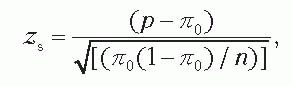
Step 5. Compute test statistic zs in terms of parameters under H0, where zs is a z-score from the standard normal distribution, and obtain the p value as twice the probability associated with the zs assuming that H0 is correct. If the significance level is .05, z0.975 is 1.96. With the wide availability of computer-based packages that contain statistical functions, many clinical investigators can obtain the p value.
where p is the estimate from the sample of the parameter π0. One should note that ; the squared z-score, obtained from the data (i.e., zs), equals a chisquare test statistic with 1 degree of freedom obtained from the same data (i.e., ). Most computer packages report a chi-square test statistic with 1 degree of freedom (i.e., ) along with the associated p value. If the significance level is .05, with 1 degree of freedom is 3.84, which equals 1.962. If the normal approximation to the binomial is not valid, p values may be obtained by the exact method.
Step 6. Decide whether to reject or fail to reject H0. Compare the p value to α.
One-Sided Hypothesis Tests If the hypothesis test is onesided (i.e., H1: π > π0), calculate power and estimate sample size substituting 1-α for 1-α/2 in the previous formulas (e.g., z0.95 is 1.645). In addition, the p value is not multiplied by 2. It is always easier to reject a one-sided test than a similar two-sided test. In addition, an effectively larger α increases power by reducing β.
Two-Sample Tests for Binomial Proportions or Rates When the random variable under study is classified into discrete categories, hypothesis testing and methods of inference should reflect the data structure. For the two-sample situation, there are two typical study designs: independent and paired samples. Before formulating the hypothesis, the investigator must determine whether the samples are independent or not. Two samples are independent when the data points in one sample are unrelated to the data points in the second sample. Samples that are not independent are paired. Paired samples may represent two sets of measurements on the same individuals. Alternatively, paired samples may represent measurements on different individuals chosen or matched such that each member of the pair is very similar to the other. Statistical analysis of data from clinical studies is valid only in the context of the study design; inferences are only valid in the context of research questions.
When a healthcare epidemiologist investigates the relationship between two dichotomous variables, the observations are tabulated in 2 × 2 tables according to attributes. For example, suppose the epidemiologist classifies observations according to the following two attributes:
Attribute 1: A,
Attribute 2: B,
The results will be classified into four groups that include all possible combinations of attributes 1 and 2: (A and B), ( and B), (A and ), and ( and ). After tabulation, data can be presented in the following format, where a, b, c, and d are the frequencies at which the four groups occur in the sample.
B
B
Total
A
a
b
a + b
c
d
c + d
Total
a + c
b + d
n
The results of studies with either independent or paired designs may be tabulated according to the frequencies into the same four groups. Thus, this table can be obtained in different ways.
Two-Sample Tests for Independent Samples Both the table and the test statistic are the same regardless of whether the data are obtained from an observational study or a clinical trial. However, the research questions, hypotheses, and statistical tests may be different depending on the type of study. Consequently, the analyses also depend on study design.
Step 1. Set up H0 and H1. In many observational studies, the investigator can only control the total number of subjects; the research question involves whether the two sets of attributes are independent of each other. The statistical test is called a test of independence or association. In observational studies, the concept of independent samples stems from the notion that for a given attribute, such as pneumonia, the patients with pneumonia are unrelated to those without pneumonia. The null and alternative hypotheses may be written as follows:
H0: π = π0 for all four groups versus H1: π ≠ π0 for at leasts one group,
where the null and alternative hypotheses are stated in terms of joint probabilities, that is, the observed proportion equals the expected proportion. The general approach is discussed in the earlier section on probability. For example, the investigator may record the observed joint probabilities of (a) developing pneumonia and being on the ventilator, (b) not developing pneumonia and being on the ventilator, (c) developing pneumonia and not being on the ventilator, and (d) not developing pneumonia and not being on the ventilator. The expected joint probabilities are those that would have occurred under the assumption of independence. The statistical test for association involves determining the probability of finding the observed joint probabilities if the attributes were independent.
For clinical trials, the general research question for studies with independent samples is whether the proportion of B (and ) is the same for A and (i.e., the proportion of patients who die is the same for those with the drug [treated] as for those without the drug [control subjects]). Usually, the investigator determines not only the total number of subjects but also the number of subjects in each group. The statistical test is called a test of homogeneity of two proportions. For example, a clinical trial of a drug that may reduce the death rate associated with ventilator-associated pneumonia may be conducted. In this example, the investigator first estimates the observed conditional probabilities of death depending on whether the subject is in the treated or the control group. Next, the investigator estimates the observed marginal probabilities of death and survival using the addition rule. Using these observed marginal probabilities, the investigator then estimates the expected conditional probabilities of death independent of whether the subject is in the treated or the control group. These expected (or theoretical) conditional probabilities are based on the assumption that the death rate is the same in both groups (i.e., that H0 is true). The statistical test involves determining the probability of finding the observed conditional probabilities if the probability of death were the same in both groups. The null and alternative hypotheses may be stated as follows:
H0:πB|A – = 0 versus H1:πB|A – = 0,
Step 2. Choose α, power, and the difference between πB|A and that is clinically meaningful.
Step 3. For clinical trials using an available computer package, determine sample size for each group, n1 and n2. Sample size is very sensitive to the difference between πB|A and πB|. This difference, also called the effect size, should be that difference which is biologically or clinically meaningful in the opinion of the researcher. When no information is available, a pilot study can be conducted to get some idea of differences that can be obtained in a particular clinical situation. Although the algebra is not difficult, the formula for determining the sample size is quite complex; the reader is referred to the formula in Sokal and Rohlf (2) or Fleiss et al. (15), which minimizes the chances of underestimating the sample size required to detect the absolute value of the difference of |πB|A − | at given levels of significance and power. The formula in Rosner (8) is used in most statistical packages and yields sample size estimates that are generally about 5% smaller than those based on the Sokal and Rohlf or Fleiss formula. Computation of sample size can be tedious. For step 3, the investigator may wish to consult a biostatistician. Computer software is available for making some computations; however, the investigator should review documentation to determine which formulas are used and choose a software package that does not typically underestimate sample size. This precaution is especially important if sample sizes are less than 50 per group.
Only gold members can continue reading. Log In or Register to continue
 ) (i.e., p1 + p2). The other total probabilities, Pr(
 ), Pr(V), and Pr(
 ), can be calculated by using the addition rule and are displayed in the following table.
 )
) and V)
 and
and  )
) )
) )
) ) × Pr(P|
 )
) |V)
|V) ) × Pr(
 |
| )
) )
) )
) |P)
|P) ) × Pr(V|
 )
) ) ×Pr(
 |
| )
) )
) ) = .167. Thus, the RR is 1.497. In this situation, the officer would conclude that according to these data, a patient on a ventilator is about 1.5 times as likely to develop pneumonia as a patient who is not on a ventilator.
 ) can be thought of as the underlying probability of not having the disease state; it is not necessarily the probability of wellness or health.
 |
| )—refers to test specificity. The sensitivity and specificity of a test are independent of prevalence.
 |D)
|D) ) × Pr(T|
 )
) ) × Pr(
 |
| )
) )
) )
) |
| )—refers to negative predictive value of the test (PV−).
 ) × Pr(D|
 )
) |T)
|T) ) × Pr(
 |
| )
) )
) )
) and D)
 )
) and
and  )
) )
) )
)
 ; the squared z-score, obtained from the data (i.e., zs), equals a chisquare test statistic with 1 degree of freedom obtained from the same data (i.e.,
  ). Most computer packages report a chi-square test statistic with 1 degree of freedom (i.e.,
  ) along with the associated p value. If the significance level is .05,
  with 1 degree of freedom is 3.84,

 and B), (A and
  ), and (
 and
and  ). After tabulation, data can be presented in the following format, where a, b, c, and d are the frequencies at which the four groups occur in the sample.
 ) is the same for A and
  (i.e., the proportion of patients who die is the same for those with the drug [treated] as for those without the drug [control subjects]). Usually, the investigator determines not only the total number of subjects but also the number of subjects in each group. The statistical test is called a test of homogeneity of two proportions. For example, a clinical trial of a drug that may reduce the death rate associated with ventilator-associated pneumonia may be conducted. In this example, the investigator first estimates the observed conditional probabilities of death depending on whether the subject is in the treated or the control group. Next, the investigator estimates the observed marginal probabilities of death and survival using the addition rule. Using these observed marginal probabilities, the investigator then estimates the expected conditional probabilities of death independent of whether the subject is in the treated or the control group. These expected (or theoretical) conditional probabilities are based on the assumption that the death rate is the same in both groups (i.e., that H0 is true). The statistical test involves determining the probability of finding the observed conditional probabilities if the probability of death were the same in both groups. The null and alternative hypotheses may be stated as follows:
 = 0 versus H1:πB|A –
  = 0,
= 0, that is clinically meaningful.
 . This difference, also called the effect size, should be that difference which is biologically or clinically meaningful in the opinion of the researcher. When no information is available, a pilot study can be conducted to get some idea of differences that can be obtained in a particular clinical situation. Although the algebra is not difficult, the formula for determining the sample size is quite complex; the reader is referred to the formula in Sokal and Rohlf (2) or Fleiss et al. (15), which minimizes the chances of underestimating the sample size required to detect the absolute value of the difference of |πB|A −
  | at given levels of significance and power. The formula in Rosner (8) is used in most statistical packages and yields sample size estimates that are generally about 5% smaller than those based on the Sokal and Rohlf or Fleiss formula. Computation of sample size can be tedious. For step 3, the investigator may wish to consult a biostatistician. Computer software is available for making some computations; however, the investigator should review documentation to determine which formulas are used and choose a software package that does not typically underestimate sample size. This precaution is especially important if sample sizes are less than 50 per group.


