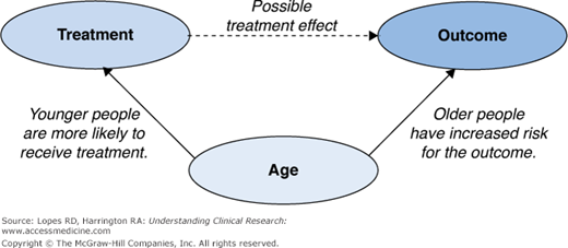
Chapter 13 discussed many of the obstacles inherent in the analysis of data from observational studies, with bias due to confounding arguably the largest of these concerns. Confounding can be seen as an issue of “mistaken identity,” in which the cause of an observed effect is attributed to the wrong party. As an example, consider a cohort study undertaken to assess the efficacy of a treatment. In this cohort, younger people are more likely to receive the treatment and are less likely to experience the outcome of interest (Figure 15–1). If a treatment effect is observed, it is unclear whether the observed effect is due to the treatment or to the younger age of the patients receiving the treatment. That is, age and treatment are said to be confounded; equivalently, age is said to be a confounder. Formally, a confounder is any variable related to both the outcome of interest and the treatment under study. In our example, age affects both the event rate and which treatment the person receives.

Throughout this chapter, we will refer to nonrandomized “treatment.” This term is not restricted to a medication; it can refer to a medical procedure or any variable of interest. The key characteristic of this “treatment” is that it was not assigned at random during the study. To facilitate discussion, we will typically consider a binary treatment; that is, patients can be divided into two treatment (or exposure) groups. Everything presented in this chapter can be generalized to the case of multiple treatment groups.

Whenever the exposure to a “treatment” is not due to randomization (such as in an observational study), confounding is likely. If we fail to address the confounding when conducting the analysis, we could mistakenly attribute an observed difference to the treatment under study when, in actuality, the difference is due to a second factor. In this chapter, we introduce several analytical approaches commonly used to address confounding. We also discuss the clinical assumptions underlying each method and common pitfalls to avoid.

Suppose a patient with a recent diagnosis of hypertension asks for a treatment recommendation. Should the physician make this recommendation without meeting with the patient? Or would he or she first want to consider the patient’s history, collect vital signs, etc.? This latter approach—making treatment decisions given certain patient characteristics—suggests a “conditional” approach to addressing confounding. That is, if treatment decisions are made conditionally, perhaps the treatment effect we are interested in estimating is the effect given other patient characteristics. This is the motivation behind regression adjustment. Although the details of regression models were covered in Chapter 14, we will briefly consider how a regression model can be used to adjust for confounding.

The concept is straightforward: include the treatment and any potential confounders (variables related to both treatment and outcome) in a regression model. The estimated treatment effect in this multivariable regression model is then adjusted for the confounders included in the model. Identifying all potential confounders is not straightforward, however. Because the issue of identifying confounders underlies each of the methods presented, we will return to it at the end of this chapter. For now, let us assume we know which variables contribute to the confounding.

Mathews et al. (1) investigated the benefit of using emergency medical services (EMS) transport versus self-transport in patients who were having acute myocardial infarction (MI). The authors first compared the “raw” or unadjusted times from symptom onset to hospital arrival between patients transported by EMS and those transporting themselves (Table 15–1), finding that people transported by EMS arrived at the hospital significantly earlier after their symptoms began than did patients who transported themselves. They then repeated the comparison after adjusting for sociodemographic factors (including age and ethnicity) and clinical factors (including systolic blood pressure and prior stroke) that each were associated with the use of EMS transport. After multivariable adjustment, EMS-transported patients were still about twice as likely as self-transported patients to arrive at the hospital within 120 minutes after symptom onset (P < 0.001). The logistic model for the probability of arriving at the hospital within 120 minutes after symptom onset included both the mode of transportation used by the patient and all confounding variables. The odds ratio associated with the mode of transportation from this multivariable model is the value reported by the authors.

The results suggest that among two patients with common values for all confounding variables, those who use EMS transport arrive at the hospital earlier, on average, than those who transport themselves. Notice that this result is interpreted as conditional on the knowledge of other variables.

One pitfall common in regression analysis is extrapolation—assuming the treatment effect is valid for a patient who is not represented in the sample. Once numerous variables are entered into a model, it can be difficult to determine when extrapolation is occurring. For example, in the EMS study above, the result might not apply to a 75-year-old white man who has not had a prior stroke if no such individual was included in the sample. Additionally, the relationship between confounders and outcome must be modeled correctly, including nonlinearity and even interactions. Although a simple model can suffice, there is no guarantee that it does, and conclusions could be erroneous if the model is not accurate.

Intuitively, if we restrict our analysis to a subgroup of patients who are similar with respect to the confounding variables, then any remaining treatment effect should not be biased. Thus, we might consider doing a separate analysis in each of these subgroups. Such a subgroup analysis, however, prevents us from using all available data. Stratification reconciles these two objectives by combining the information from each subgroup to develop a better estimate of the treatment effect. This approach has three steps: (1) divide the sample into groups (or “strata”) that have similar values of the confounders, (2) run the analysis in each group, and (3) combine the results to obtain an overall estimate of the treatment effect. This approach is valid if the treatment effect is believed to be similar within each group, and there are no remaining differences between patients that could confound treatment within the strata.

Consider a hypothetical study in which investigators use an existing trial database to compare the efficacy of two treatments in reducing the rate of MI 30 days after percutaneous coronary intervention (PCI). The data include patients for whom treatment was assigned at the discretion of the physician. It is known that diabetic patients were more likely to receive Treatment A, but there were no other characteristics associated with treatment. We believe that the treatment should have the same effect in diabetic patients as in nondiabetic patients. To adjust for the confounding via stratification, we compute the treatment effect for diabetic and nondiabetic patients separately; then we combine the results to get an overall treatment effect. This process is illustrated in Figure 15–2.

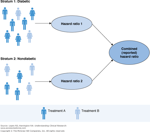
Note that this is not a subgroup analysis. The effect within each stratum is not reported separately; the stratification is used only to adjust for the confounding, and the final pooled estimate is of singular interest. Although stratification is intuitive, it can become complicated to implement as the number of confounders grows, because we need to identify multiple patients assigned to each treatment that will fall within a given strata. In the example above, we identified diabetic patients who were assigned Treatment A and diabetic patients who were assigned Treatment B (similarly for nondiabetics). However, suppose we stratified on diabetic status, sex, race, and age. It can be very difficult to find multiple patients taking Treatment A and multiple patients taking Treatment B who are diabetic, female, Caucasian, and more than 65 years old.

As with regression analysis, the estimate obtained from stratification is conditionally interpreted as the effect among individuals with common values for all strata variables. The conditional approach is powerful, but the results do not mimic those of a clinical trial. Clinical trials assess the “marginal” effect—the treatment effect that we might expect to see on average in the population. It is natural to then question which interpretation is best, conditional or marginal. When the goal of a study is to establish that a treatment effect exists, a distinction between these interpretations is rarely made. Although the resulting estimate may differ depending on the method chosen, the direction of the effect and its significance are not likely to change. Therefore, the effect of a treatment can be established using either approach. However, care should be given to the desired interpretation before a method is chosen.

We can think of extending stratification in such a way that exactly two patients (one from each treatment group) fall into each stratum. This leads to matching. As the name implies, matching involves pairing patients in one treatment group with those in the other who are similar. Patients should be matched with respect to confounding variables. That is, each patient in one treatment group is paired with a patient in the other treatment group who has similar values for the confounding variables. Matching can be a part of the data collection, or it can take place afterward; however, it is much easier to ensure good results in the former case. Thus, it is important to have a statistician involved during the early phases of the study design and data collection.

Suppose you would like to use data collected in a registry to compare the efficacy of two treatments in reducing mortality at 30 days after treatment. You have identified patients who received Treatment A, the treatment of interest. Further, you know that sex and diabetes status are potential confounders and would like to account for these via matching. For each of the patients who received Treatment A, you must identify a patient from the registry who received Treatment B (the competitor) who is of the same sex and diabetes status. This process will create two groups that are similar with respect to the variables used in the matching process (sex and diabetes in this case), as illustrated in Figure 15–3. Differences between the matched groups cannot be attributable to sex or diabetes, because the groups are similar in these features. When no other confounders exist, differences must be attributable to treatment.