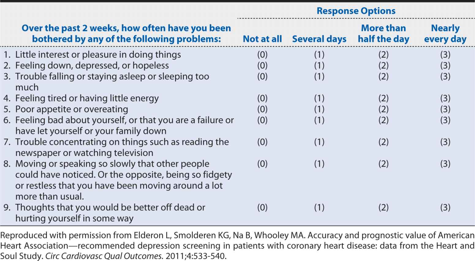
A slightly more detailed screening instrument for depression is the nine-item Patient Health Questionnaire (PHQ-9). The questions that are included in this instrument are shown in Table 10-2. The nine-item version collects basic information on each of the potential manifestations of major depressive disorder cited in the DSM definition. Clearly, it requires longer than the two-item version, but it still can be self-administered or conducted by a clinician relatively quickly and inexpensively compared with a much more detailed clinical interview. The obvious question is whether such a condensed and concise screening instrument can provide an accurate characterization of depression status. The savings in time, money, and burden on patients and staff would not be justified if the PHQ-2 and PHQ-9 led to incorrect conclusions about which patients are experiencing depression. In the following sections, we will explore how one can assess the performance of a screening test. These methods can be applied to screening and diagnostic tests regardless of whether they are obtained from a questionnaire, a blood test, a radiologic examination, or a surgical biopsy.
Table 10-2. Questions on the nine-item Patient Health Questionnaire (PHQ-9).
SENSITIVITY AND SPECIFICITY
To characterize the ability of the PHQ-2 to identify patients with a major depressive disorder and separate them from those without such a disorder, Elderon and colleagues (2011) conducted a study of more than 1000 patients with heart disease. Every patient completed the screening instrument and that same day separately underwent a structured computerized, diagnostic interview, which represented the “gold standard” for making a diagnosis of a major depressive order according to the criteria of the DSM. For simplicity, patients were classified in a simple dichotomous manner (screen positive vs. screen negative and depression present or absent). For each patient, one can imagine four possible combinations of screening test results and depression diagnoses:
a. Screening test positive; depression present
b. Screening test positive; depression absent
c. Screening test negative; depression present
d. Screening test negative; depression absent
As the results accumulate within the patient population, one can summarize the findings in a simple tabular format, as shown in Table 10-3. Here, the “true” disease status is defined by the gold standard method, in our example, the computerized, structure diagnostic interview. In the cell labeled a in Table 10-3, we include all patients who had a positive screening test result (e.g., PHQ-2) and had the disease of interest (e.g., major depressive disorder) according to the gold standard diagnostic method. For these patients, the screening test identified their disease status correctly, so we refer to these individuals as “true positives.” If we consider the group diagonally opposite—those who had negative screening results and did not have the disease of interest—again, the screening test performed correctly, and we refer to these individuals as “true negatives.”
Table 10-3. Tabular summary of the findings of a comparison of screening test results with the “true” status of disease.
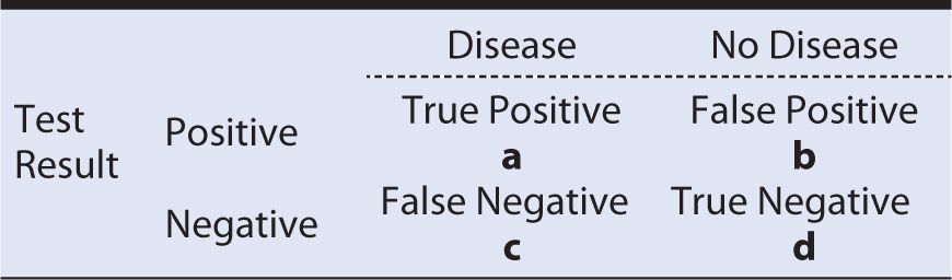
In the remaining two cells of Table 10-3, we have the situations, where the screening test incorrectly classified persons. For example, in cell b, the patients had positive test results but did not have the disease of interest. We refer to these individuals as “false positives” because the screening test falsely indicated the presence of disease. In the final cell, c, we have the individuals who had negative test results but truly had the disease of interest. We refer to these individuals as “false negatives” because the screening test falsely indicated the absence of disease.
It should be readily apparent that a screening test that is highly accurate in classifying persons with regard to disease status will tend to place subjects into cells a and d, where disease status is classified correctly. This also implies that errors are being made less often, so cells b and c will tend to have fewer occupants. Indeed, if the test was perfect at discriminating between truly affected and unaffected individuals, all of the results would fall into cells a and d, with none in b and c. Unfortunately, even the best screening tests occasionally make mistakes, so we need a way to quantify the extent to which the test is classifying subjects correctly. We begin with two basic measures that are commonly used to describe test performance—sensitivity and specificity.
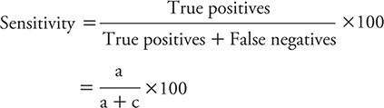
The sensitivity of a test is the percentage of persons with the disease of interest who have positive test results. We might express this concept mathematically as:
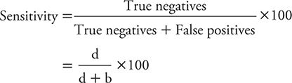
The specificity of a test is the percentage of persons without the disease of interest who have negative test results. The formula for calculating specificity is:
Example: The previously mentioned study of Elderon and colleagues (2011) was designed to explore the relationship between depression and cardiovascular disease among patients. They included more than 1000 patients from two U.S. Department of Veterans Affairs hospitals, a university hospital, and nine public health clinics. The enrolled patients underwent an initial examination and were followed annually thereafter through telephone interviews.
Several instruments were used to screen for depression, including the previously cited PHQ-2 and PHQ-9. As the “gold standard” for making a diagnosis of major depressive disorder, the investigators used a structured Computerized Diagnostic Interview Schedule (C-DIS), which requires trained personnel to administer and can take 1 hour or longer to complete.
When compared against the “gold standard” C-DIS, the quick screen PHQ-2 yielded the results shown in Table 10-4. From these data, we can see that sensitivity is:
![]()
Table 10-4. Tabular summary of the findings of a two-item Patient Health Questionnaire (PHQ-2) screening test versus a diagnostic interview (Computerized Diagnostic Interview Schedule [C-DIS]).
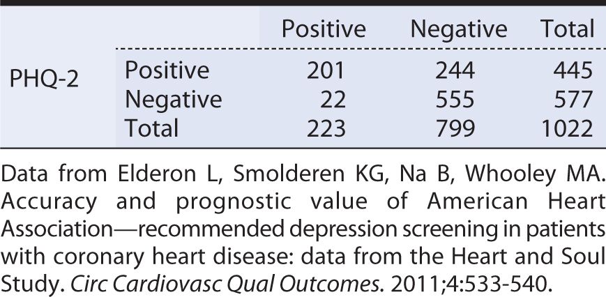
This is relatively high sensitivity, meaning that the PHQ-2 is reasonably good at detecting persons with major depressive symptoms. Because the test identifies most depressed persons, a negative test result helps to “rule out” or lower the suspicion that the individual in question truly is depressed.
The specificity of the PHQ-2 is calculated as:
This specificity is not particularly high, meaning that a positive test result does not allow us to “rule in” or conclude with high confidence that the person in question truly is depressed.
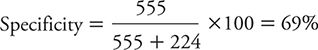
Elderon and colleagues (2011) also evaluated the sensitivity and specificity of the PHQ-9, again using the C-DIS as the “gold standard.” The results of this comparison are summarized in Table 10-5. Here, the sensitivity is:
![]()
Table 10-5. Tabular summary of the findings of the a two-item Patient Health Questionnaire (PHQ-2) screening test versus a diagnostic interview (Computerized Diagnostic Interview Schedule [C-DIS]).
This sensitivity is not nearly as high as that previously noted for the PHQ-2. In other words, the PHQ-9 is more likely than the PHQ-2 to miss some persons who truly are depressed. A negative test result, therefore, would not be as helpful in ruling out depression.
The specificity of the PHQ-9 was:
![]()
When compared against the PHQ-2, the PHQ-9 had a much higher specificity, meaning that it is more helpful in “ruling in” depression in a person with a positive test result.
Given the differing characteristics of the PHQ-2 and the PHQ-9, it is reasonable to ask which screening test is preferred. On one hand, the PHQ-2 does a better job at detecting depressed persons than does the PHQ-9. The price for missing fewer affected persons is that the PHQ-2 also has a greater tendency than the PHQ-9 to falsely label nondepressed people as having depression. When the condition of interest is serious, and if undetected, leads to life-threatening consequences, one might prefer to err on the side of overdiagnosis. However, when falsely labeling someone as affected can lead to a serious emotional toll on the patient or treatment that has significant cost and potential side effects, one might prefer to err on the side of underdiagnosis. In the case of depression and cardiovascular disease, the AHA recommends a two-step screening process. First, the PHQ-2 is used, picking up most persons who are truly depressed. The persons who test positive on the PHQ-2 then are screened with the PHQ-9, and those who are positive are treated for depression.
POSITIVE AND NEGATIVE PREDICTIVE VALUE
Sensitivity and specificity are characteristics of screening or diagnostic tests, such as the PHQ-2 and the PHQ-9. Two other measures are helpful in assessing how a test performs within a specific population, such as patients with CAD. These two measures are, respectively, positive predictive value (PV+) and negative predictive value (PV–).
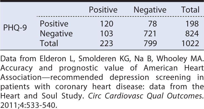
The PV+ is defined as the percentage of persons with positive test results who actually have the disease of interest. In other words, PV+ tells us the implications of a positive test in terms of the likelihood of having disease (e.g., depression). The PV+ is calculated as follows, using the same symbolic notation found in Table 10-3.
Using the findings of Elderon and colleagues (2011), for PHQ-2 as an example (see Table 10-4), the PV+ is calculated as:
![]()
In other words, slightly less than half of the persons who had a positive PHQ-2 in the population studied by Elderon and colleagues (2011) actually had depression. At first impression, getting a positive result on a PHQ-2 screen may seem no more predictive than flipping a coin. It is worth considering, however, what our baseline expectations was for depression in this population before conducting the PHQ-2.
In the patients that Elderon and colleagues (2011) studied, the prevalence of depression as identified by the “gold standard” C-DIS was:
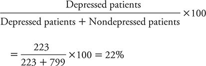
So, for patients who have positive results on the PHQ-2, the likelihood of being depressed rises from the pretest likelihood of 22% to 45%. That is, a positive test result raises the likelihood that depression is present twofold. So, even though the test is making a lot of mistakes, it is still improving one’s ability to identify depressed patients.
The PV- is defined as the percentage of persons with negative test results who do not have the disease of interest (e.g., depression). One can calculate the PV– using the symbolic notation introduced in Table 10-3 as:
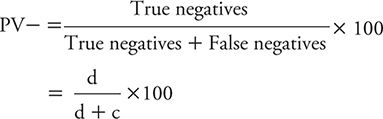
We can illustrate the calculation of the PV– using the data for PHQ-2 from Elderon and colleagues (2011), as shown in Table 10-4:
In other words, in this patient population, a negative test result for a patient makes it very unlikely that he or she is depressed. Another way of looking at this is that the pretest probability of not being depressed (799 of 1022) rises from 78% to the posttest probability of 96% if a patient has a negative PHQ-2 result.
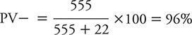
The PV+ and PV– vary according to the baseline risk (prevalence) of the condition of interest in the population being studied. Patients with cardiac disease are at relatively high risk for depression, as reflected by the 20% prevalence of depression in the heart disease patients studied by Elderon and colleagues (2011). Surveys of the general adult population typically reveal a prevalence of 10% or less. To explore how PV+ and PV– vary as a function of prevalence, we can consider a study analogous to the one presented by Elderon and colleagues (2011), but instead of studying heart patients, the focus was on adults in the general population. For this exercise, let us assume that the same number of subjects (n = 1022) was studied, the PHQ-2 had the same sensitivity (90%) and specificity (69%), and the prevalence of depression according to the C-DIS is 10%. We can use this information to complete a display of hypothetical test results (Table 10-6) in the following manner.
Table 10-6 Hypothetical data for a study of the Patient Health Questionnaire (PHQ-2) screening test for depression in the general population (prevalence of depression = 10%; sensitivity = 90%; specificity = 69%).
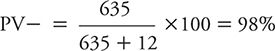
With a prevalence of 10%, the total number of C-DIS positive individuals is 102 (1022 × 0.10), and the remainder (1022 – 102 = 920) are C-DIS negative. Applying a sensitivity of 90% to the 102 C-DIS positive persons yields a true positive number of 90, with the balance (102 – 90 = 12) being false negatives. Applying the specificity of 69% to the total of 920 C-DIS negative persons yields a number of true negatives of 635, with the balance (920 – 635 = 285) being false positives.
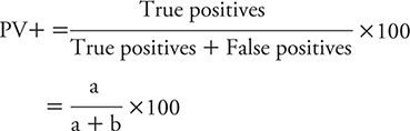
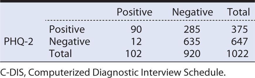
From the hypothetical data calculated and displayed in Table 10-6, we can now calculate a PV+ and PV–. The PV+ is:
![]()
The PV– can be calculated as:
If these results are compared with those obtained by Elderon and colleagues (2011) among cardiac patients, one can see the impact of lowering disease prevalence (or alternately expressed, disease risk) on PV+ and PV–. The PV+ dropped from the original 45% among heart patients to 24% in the hypothetical general population because prevalence declined from 20% to 10%. In contrast, PV– rose from the original 96% among cardiac patients to 98% within the hypothetical general population.
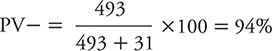
However, if we studied an even higher risk group for depression than cardiac patients in general, we would expect to see PV+ and PV– move in the opposite directions. For example, suppose we identified a subset of heart patients who were either older or had more extensive disease; we might expect such a group to have a higher prevalence (e.g., 30%) of depression than among heart patients in general. If one goes through the same sort of hypothetical exercise, a study of 1022 total subjects would yield 307 depressed persons (1022 × 0.30 = 307), 276 true positives (307 × 0.90 = 276), 31 false negatives (307 – 276 = 31), 715 nondepressed persons (1022 – 307 = 715), 493 true negatives (715 × 0.69 = 493), and 222 false positives (715 – 493 = 222). The PV+ would be calculated as:
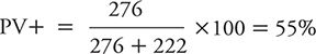
The PV– would be calculated as:
So, we see that as prevalence rises (i.e., we examine higher risk persons), the PV+ increases, and the PV– decreases.
CUTOFF POINTS
Thus far, we have presented the concepts of screening and diagnostic tests as simple positive or negative results. In medicine, it is common practice to measure attributes in a simple dichotomous fashion, such as normal versus abnormal. Advantages of a binary classification (e.g., yes/no, or present/absent) include that it is easy to communicate and understand. However, it may lack some of the detail that can be found in measures of progressive ordered categories or continuous results. For characteristics that have multiple levels, such as questionnaires about depressive symptoms, an interesting question arises around where one should draw the cutoff point or dividing line between normal and abnormal results.
To illustrate the impact of changing cutoff points for defining an abnormal test result, consider a study published by Zuithoff and colleagues (2010). This investigation involved more than 1300 patients older than age 18 years who were sampled from seven large primary care practices in the Netherlands. Patients were enrolled regardless of their reasons for seeking medical care. Each patient completed the PHQ-9, and the “gold standard” was the Composite International Diagnostic Interview, a standardized, structured interview administered by trained researchers. The PHQ-9 was scored according to the numerical method shown in Table 10-2, with each of the nine questions scored from 0 to 3 depending on symptom frequency. Aggregate scores, therefore, could range from a minimum of zero (no depressive symptoms) to a maximum of 27 (all nine symptom categories experienced nearly every day).
Overall, 13% of the patient population had a major depressive disorder according to the reference standardized structured interview. The observed sensitivity and specificity of the PHQ-9 for detecting major depressive disorder are shown in Figure 10-1 for varying cutoff points. In general, as the cutoff point is raised (more symptoms or greater frequency required to declare a positive test result), the sensitivity falls. That is, as it becomes more difficult to be classified as abnormal, the screening test misses more and more truly depressed persons (i.e., the false-negative rate increases, and the sensitivity falls). However, as the threshold for an abnormal result rises, there is a corresponding progressive increase in specificity. That is, as it becomes more difficult to be classified as abnormal, the screening test produces fewer and fewer false positives.
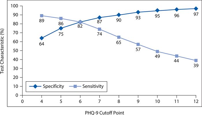
Figure 10-1. Changes in sensitivity and specificity of the nine-item Patient Health Questionnaire (PHQ-9) as a function of changing the cutoff point. (Data from Zuithoff NPA, Vergouwe Y, King M, et al. The Patient Health Questionnaire-9 for detection of major depressive disorder in primary care: consequences of current thresholds in a cross-sectional study. BMC Family Pract. 2010;11:98.)
It can be seen that neither the fall in sensitivity nor the rise in specificity is linear. For the decline in sensitivity, the greatest incremental losses occur between cutoff points of 6 and 10. In contrast, the greatest gains in specificity occur between cutoff points of 4 and 7.
Choosing the optimal cutoff point requires a judgment about the relative consequences of a false-positive and a false-negative error. The kinds of issues that must be considered are whether it is worse to miss a diagnosis of depression (false negative) and thereby have less effective treatment or to mistakenly label a person as depressed (false positive), leading to perceived or real social, employment, or emotional stigma, as well as extra testing and unnecessary treatment. In general, the relative gains in specificity seem to be a reasonable offset to the losses in sensitivity when moving the cutoff point from 4 to 6 or 7. Raising the cutoff point above that level would require a decision that modest reductions in false-positive errors were warranted by greater inflation of false negative errors. It should be noted in this context that a widely recommended and used cutoff point for the PHQ-9 is 10. In deploying this cutoff point, the user should be aware that it entails lower sensitivity than could be achieved with a slightly lower cutoff point.
LIKELIHOOD RATIOS
In addition to the metrics already introduced, screening or diagnostic tests often are assessed with likelihood ratios (LRs). An LR is the probability for a particular test result for a person with the condition of interest (e.g., depression) divided by the probability of that test result for a person without the condition of interest. We can further specify an LR for a positive test result (LR+) as the probability of a positive test result for a person with the condition of interest divided by the probability of a positive test result for a person without the condition. The mathematical expression for the LR+, where sensitivity and specificity are expressed as proportions (rather than as percentages) is:
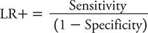
Consider the possible range of the LR+. It is minimized when the numerator (sensitivity) is zero. It is maximized when the denominator is zero (specificity = 1). An LR+ = 1 implies that the test does not perform better (i.e., more likely to yield a positive result) among affected persons than among nonaffected persons. In other words, the test is not helpful in sorting out affected persons from unaffected persons. A value greater than one for LR+ implies that a positive test result is more likely when the condition is present, and the larger the LR+, the more a positive test result is indicative of having the condition of interest.
The LR for a negative test result (LR–) is defined as the probability of a negative test result for a person with the condition of interest divided by the probability of a negative test result for a person without the condition. The LR– is calculated as:
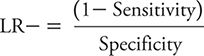
Sensitivity and specificity again are expressed as proportions. The smallest possible value of LR– (= 0) occurs when the numerator is zero, meaning that 1 – sensitivity = 0, so sensitivity = 1. The largest possible value of the LR– occurs when the denominator has its smallest possible value. This occurs when the specificity is zero, resulting in an LR– of positive infinity.
As was the case with the LR+, an LR– with a value of one indicates a test with no discriminatory value. When the LR– is 1, people with and without the condition of interest are equally likely to have a negative test result. A test that is more likely to be negative in the absence of the condition of interest will have an LR– value less than 1, and the further from 1, the stronger the association between a negative test result and the absence of disease.
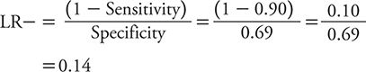
The calculation of LR+ and LR– can be illustrated for PHQ-2 and PHQ-9 using the data previously cited in Tables 10-4 and 10-5 based on the study of Elderon and colleagues (2011). For PHQ-2, sensitivity is 0.90, and specificity is 0.69.
The LR+, therefore, is calculated as:
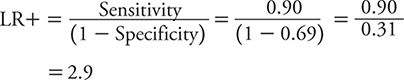
The LR– is calculated as:
For PHQ-9, sensitivity is 0.54, and specificity is 0.90.
Accordingly, LR+ is:
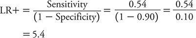
LR– is:
So, how does one interpret these LRs? With an LR+ of 2.9, a positive test result on the PHQ-2 only raises the likelihood of depression a small amount compared with a positive result on the PHQ-9 (LR+ of 5.4), which raises the likelihood of depression a moderate amount. However, a negative test result on the PHQ-2 (LR– = 0.14) conveys a moderate decrease in the likelihood of depression compared with a minimal decrease associated with a negative test result on the PHQ-9 (LR– = 0.51). Neither test has the kind of strong discriminatory power that one would like to see to either confirm a diagnosis of depression or exclude it. To “rule in” or confirm a diagnosis, an LR+ of 10 or greater typically is expected. To “rule out” or exclude a diagnosis, an LR– of 0.10 or less typically is expected. With these criteria in mind, neither the PHQ-2 nor the PHQ-9 is sufficient to rule in depression, but a negative test result on the PHQ-2 is pretty compelling evidence that depression is unlikely.
RECEIVER OPERATING CHARACTERISTIC CURVES
In the preceding section on cutoff points, we saw how sensitivity and specificity varied inversely as the cutoff point for a positive test result on the PHQ-9 varied. This relationship was illustrated in Figure 10-1. Another approach to illustrating this phenomenon is referred to as the receiver operating characteristic (ROC) curve. The first use of such a graph, and hence its unusual name, arose in the context of assessing the ability of radar operators to distinguish signals from background noise. In relation to diagnostic or screening tests, we plot sensitivity on the vertical axis against 1 – specificity on the horizontal axis. It may be helpful to think of this graph as depicting the proportion of true positives (sensitivity) as a function of the proportion of false positives (1 – specificity). If a diagnostic test has no discriminating value in helping to make a diagnosis, then the true positive proportion will be identical to the false positive proportion. This line of “no value” would appear as a diagonal at a 45-degree angle and often is depicted in an ROC curve as a reference for comparing against the actual test results. A diagnostic test that helps to separate persons with and without the condition of interest would appear as a departure from this “no value” reference line, and the greater the departure, the better the test performs at distinguishing affected from unaffected persons.
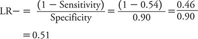
We can construct an ROC curve using the data from Zuithoff and colleagues (2010), as shown in Figure 10-2. The solid line in this graph represents the performance of the PHQ-9, and the dotted line corresponds to the reference of a test with no diagnostic value. We can see that the Sensitivity rises rapidly at the far left of the graph, with small increases in 1 – specificity (i.e., with decreases in specificity). The curve begins to flatten out as it moves to the right. In other words, in this region, there are diminishingly small gains in sensitivity for the corresponding losses in specificity.
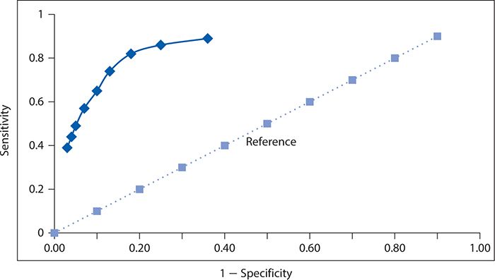
Figure 10-2. Receiver operating characteristic curve for the nine-item Patient Health Questionnaire. (Data from Zuithoff NPA, Vergouwe Y, King M, et al. The Patient Health Questionnaire-9 for detection of major depressive disorder in primary care: consequences of current thresholds in a cross-sectional study. BMC Family Pract. 2010;11:98.)
A summary measure of overall test performance can be calculated as the area under the ROC curve. The minimal value of this measure is 0.5, which corresponds to the area under the dashed diagonal line in Figure 10-2, which reflects a test of no value in distinguishing between persons with and without the condition of interest. The maximum value of the area under the ROC curve is 1, which represents a perfect test in which no errors are made. The closer the area under the ROC curve is to 1, the better the test is performing. For the PHQ-9, values of the area under the ROC curve have been reported in the range of 0.85 to 0.90 or higher depending on the setting and study population.
The performance of two screening or diagnostic tests can be compared visually, as illustrated with hypothetical data in Figure 10-3. Here, test A has a steeper ascent and reaches a higher sensitivity level than does test B. It is readily apparent that the corresponding area under the ROC curve will be greater for test A than for test B, and thus, test A performs better at screening for depression.
Figure 10-3. Contrast of two different screening tests (A and B) for depression with respective receiver operating characteristic curves, with the dotted line corresponding to a reference test with no diagnostic value.
EARLY DETECTION BIASES
Screening tests typically are used to detect a condition earlier than it might otherwise come to recognition through clinical manifestations (symptoms) of the disease. The benefit of early detection is that it allows earlier intervention to either prevent the condition from developing fully or allowing it to be treated at a stage when the condition is more limited and curable. Of course, the benefits will be achieved only if effective treatments are available and if there are therapeutic advantages to early intervention. Examples of screening tests that have been shown to be effective and are widely recommended include the Pap smear for cervical cancer, fecal occult blood screening, sigmoidoscopy and colonoscopy for large bowel cancer, and serum lipid screening for elevated total cholesterol and low density lipoprotein-cholesterol and decreased levels of high density lipoprotein-cholesterol as risk factors for coronary heart disease.
Studies conducted to evaluate the effectiveness of a screening test must take into account several factors that may influence the results. The first of these influences has been referred to as lead time bias. The lead time is the extra amount of time that a condition is recognized by early detection through screening. For an individual, it begins when the condition is screen-detected and ends when it would be detected in the absence of screening. If one were assessing the effectiveness of a screening test by the extra amount of time that screen-detected persons survive, the lead time would make their survival appear longer than non–screen-detected persons even if there is no prolongation of life. That is, the clock is starting at unequal points in time for screen-detected and non–screen-detected persons, and if an adjustment is not made for this “head start” with screening, the comparison will be unfair.
Yet another type of unfair comparison might arise from so-called length-biased sampling. The length bias arises because slowly progressing forms of a condition are detectable by the screening test for a longer period of time than rapidly progressing forms. The subset of affected individuals that the screening test detects, therefore, likely will be weighted preferentially to nonaggressive slowly developing forms of the disease. If one assesses the effectiveness of screening by duration of survival, the screen-detected persons will appear to live longer than non–screen-detected persons because they tend to have slower progressing forms of the condition.
To reduce the risk of both lead time bias and length-biased sampling, it is recommended that the evaluation of screening effectiveness should be determined by a comparison of cause-specific mortality rates for the condition of interest. The strongest evidence would derive from a controlled clinical trial in which subjects were randomly assigned to the screening program or no screening.
SUMMARY
In this chapter, we used the example of screening for depression among persons with CAD to present the basic concepts of diagnostic testing. Central to this discussion is the understanding that all clinical information, including information that results from diagnostic tests, is subject to error. We introduced the concept of a false-negative result in which a test does not detect the condition of interest when it is present. We also learned about a second type of error, a false-positive result, which occurs when the diagnostic test mistakenly indicates that the condition of interest is present when it is not.
Applying these concepts, we learned that sensitivity is the proportion of positive test results among all persons with the condition. Specificity relates to the proportion of negative test results among persons without the condition. A test is said to be sensitive when it correctly detects a high proportion of truly affected persons. A test may be described as specific when it correctly provides negative results for a high percentage of unaffected persons. Applying these criteria to screening for depression, we saw that the two-question PHQ was sensitive but not very specific, and the nine-question PHQ was specific but not very sensitive.
Positive predictive value (PV+) characterizes the proportion of persons with positive test results who truly are affected with the condition of interest. The companion measure, negative predictive value (PV–), corresponds to the proportion of persons with negative test results who truly lack the condition of interest. We saw that among cardiac patients, in whom the risk of depression is higher than in the general population, the two-question PHQ had a PV+ of 45% and a PV– of 96%. Accordingly, one would expect the PV+ to be lower and the PV– to be higher if the PHQ two-question test for depression was used in a lower risk group (e.g., the general population). The reverse would be true if the PHQ-2 was applied to a higher risk subgroup (e.g., older patients with coronary heart disease or those with greater morbidity).
Next, we examined the impact of changing the cutoff point for declaring a test result to be positive. In general, as one raises the cutoff point, the criteria for a positive result become more difficult to achieve. This will result in a greater proportion of truly affected persons being missed (declared negative) by the test, raising the false-negative rate, or said another way, lowering the sensitivity. Typically, the loss of sensitivity will be accompanied by a drop in false positives, or a rise in specificity. We observed these impacts on the sensitivity and specificity of the nine-question PHQ as a function of raising the cutoff point.
We then considered two further measures, which are termed likelihood ratios (LRs). The LR+ is the probability of a positive test result for a person with the condition of interest divided by the probability of a positive test result for a person without the condition. The LR– is the probability of a negative test result for a person with the condition of interest divided by the probability of a negative test result for a person without the condition. Applied to the PHQ tests, a negative test result on the two-question version conveys a moderate reduction in the likelihood of depression. A positive test result on the nine-question version raises the likelihood of depression to a moderate extent.
The concept of the ROC curve was introduced as a way to depict a visual image of the discriminatory ability of a diagnostic test. Furthermore, one can use such an image to compare and contrast the performance of two or more diagnostic tests and a summary measure of performance can be calculated as the area under the ROC curve.
Finally, we saw how the evaluation of a screening test can be distorted by two different types of effects. Lead time bias is the apparent increase in survival with screening that is attributable to the time differential related to earlier diagnosis through screening than through nonscreened diagnosis. Length-biased sampling relates to the fact that screen-detected disease may be skewed toward slower progressing forms of the condition, resulting in a survival advantage compared with patients diagnosed through nonscreened methods. Both types of distortion can be removed by focusing on cause-specific death rates rather than survival time in a controlled clinical trial where screening is assigned randomly.

1. In raising the cutoff point for a screening test, which of the following is the likely result?
A. An increase in sensitivity
B. An increase in specificity
C. An increase in false positives
D. An increase in prevalence
E. An increase in lead time bias
2. If the screening test does not delay the time of death from a condition but makes survival appear longer because of earlier detection of disease, there is evidence of
A. confounding.
B. length-biased sampling.
C. lead time bias.
D. selection bias.
E. information bias.
3. A test with an LR+ of 15 can be said to provide evidence to
A. rule in the condition of interest.
B. rule out the condition of interest.
C. make an earlier diagnosis.
D. prolong survival after diagnosis.
E. detect slowly progressing forms of the condition of interest.
4. A specific diagnostic test is one that
A. has a high proportion of false-negative results.
B. has a low proportion of false-negative results.
C. has a high proportion of false-positive results.
D. has a low proportion of false-positive results.
E. none of the above.
5. A diagnostic test with no discriminatory ability would have an area under the ROC curve of
A. 0.
B. 0.25.
C. 0.5.
D. 1.
E. 2.
6. A diagnostic test with an LR- of 0.05 can be said to provide evidence to
A. rule in the condition of interest.
B. rule out the condition of interest.
C. make an earlier diagnosis.
D. prolong survival after diagnosis.
E. detect slowly progressing forms of the condition of interest.
7. If a screening test does not delay the time of death from a condition but makes survival appear longer because it is preferentially detecting slowly progressing disease, there is evidence of
A. confounding.
B. length-biased sampling.
C. lead time bias.
D. selection bias.
E. information bias.
8. Two screening tests are being compared for a particular disease. Test A has an area under the ROC curve of 0.95. Test B has an area under the ROC curve of 0.83. Which of the following statements is correct?
A. Neither test has any discriminatory value.
B. Test A has a total error rate of 5%.
C. Test B is better than test A at ruling in disease.
D. The PV+ for test A is 95%.
E. Test A performs better than test B at discriminating the presence of disease.
9. As the prevalence of a condition increases, a screening test for it will tend to have a
A. higher sensitivity.
B. higher specificity.
C. higher predictive value positive.
D. higher predictive value negative.
E. higher length biased sampling.
10. Which of the following measures of diagnostic test performance ideally has a small value?
A. Predictive value positive
B. Predictive value negative
C. Likelihood ratio for a positive test result
D. Likelihood ratio for a negative test result
E. None of the above
Stay updated, free articles. Join our Telegram channel

Full access? Get Clinical Tree


