Figure 9-1. Illustration of the design of a case-control study. Shaded areas represent exposed persons, and unshaded areas represent unexposed persons.
The general design of a case-control study shown in Figure 9-1 can be illustrated by a study of LBW and CKD. The investigator would initiate such a study by identifying either newly diagnosed (incident) or existing (prevalent) cases of CKD. She would then proceed to collect information on exposure (LBW) from subject recall, or preferably, birth records or registration data, if available. In the next sections, we will consider each of these steps in greater detail.
Cases
The sampling of cases is one of the first steps in conducting a case-control study. The investigator must begin by defining the criteria for establishing what constitutes an affected individual. In some instances, it may be relatively clear how to diagnose the condition of interest. For example, many forms of cancer require a histologic confirmation of diagnosis to establish the presence of the disease of interest. As already mentioned, CKD is a spectrum of illness that stretches from asymptomatic mild impairment to severe, end-stage disease. Fortunately, there are standardized criteria for establishing a diagnosis and further categorizing the stages of illness. It should be evident that patients with more severe manifestations of illness are more likely to come to clinical recognition. This may not be a concern for a case-control study if the exposure is equally linked to all stages of illness. In some situations, however, there may be reason to believe that the disease associated with a particular exposure is either very mild or very severe. In such a circumstance, studying a limited range of disease severity in a case-control study may either miss or overstate the magnitude of the association between exposure and disease. To avoid such a problem, the investigator in a study of CKD may need to find affected individuals who have not otherwise come to medical attention already. For example, one might identify individuals in stage 1 CKD through a community-based screening program.
When affected individuals become symptomatic and seek medical care, the process of identifying them becomes more straightforward. Traditional sources of information for finding cases include medical records in hospitals and outpatient clinics, laboratories and other diagnostic facilities, reimbursement data, and other registration systems.
Equally important to establishing the definition of a case is to identify the sampling frame from which cases will be selected. At least two different general approaches warrant further discussion. One is to choose a hospital-based sample, which generally means finding the cases from the records of one or more treating facility. The advantages of this approach are that it is efficient, cost effective, and fast. It can also simplify the selection of controls if they are sampled from other patients (without CKD) who are treated at those same facilities.
These pragmatic advantages of a hospital-based case-control study must be weighed against several disadvantages. First, as already mentioned, it tends to select a sample of affected individuals who are symptomatic and have sought care. Those who are either asymptomatic or symptomatic but have poor access to care (generally associated with lower socioeconomic status) are less likely to be included. Second referral patterns to hospitals can be quite selective and could result in a skewed sample of patients at any particular facility. For example, public hospitals may tend to treat more low-income or uninsured patients. Teaching hospitals may tend to have more patients with unusual or severe forms of disease. These selection factors can be minimized somewhat by including multiple hospitals with differing referral patterns. Ideally, the inclusion of all hospitals in a region would tend to minimize selective inclusion of affected patients. Choosing controls from the same hospitals tends to control for differential referral patterns because, presumably, they would be similar for cases and controls admitted to the same hospitals. Choosing controls in a hospital-based case-control study has its own issues, which will be discussed in the next section.
The counterpart to a hospital-based case-control study is a population-based case-control study. Here, the intent is to identify all of the cases that arise within a population. Typically, the population is defined by place of residence, such as within a particular city, region, or state. The population could be defined by other parameters, however. For example, one could select the population of interest on the basis of occupation or participation in a particular health insurance plan. A population-based study has the advantage of potentially more complete case finding and avoiding potential pitfalls of referral patterns. Because controls can be selected from the same well-defined source population, they may constitute a more representative and unbiased comparison group. The challenges of a population-based study are pragmatic concerns, such as potentially greater time and expense to complete.
Controls
Although the selection of cases may seem to be the complicated sampling issue in a case-control study, it turns out that there are at least as many considerations in the selection of controls. The guiding principle for control selection is that they should come from the same population as gave rise to the cases. Another way of expressing this concept is to choose controls who would have been included as cases, had they developed the disease of interest. For population-based studies, there are a variety of methods to choose controls at random from the general population. One can use census data, or alternatively, tax records, driver’s license registration, random telephone calling, or a variety of other methods. The key issues are to use a source that has complete or nearly complete enumeration of the population and a sampling strategy that gives all eligible persons an equal chance to be selected.
For hospital-based studies, as already indicated, controls can be selected from among other patients treated at the same facilities. This tends to reduce or eliminate any distortion that might arise from selective referral patterns to the facilities of interest. Among the many patients treated at the hospital(s) included, however, how does one choose which individuals to enroll as controls? One wants to avoid any diagnosis that shares risk factors with the disease of interest. So, for example, in a hospital-based case-control study of LBW and CKD, one would want to avoid sampling controls from patients who have risk factors for CKD, such as hypertension or diabetes, or conditions related to them, such as coronary heart disease, stroke, peripheral vascular disease, retinopathy, or neuropathy. In a study of LBW as the exposure, it also would be important to avoid sampling controls from conditions known to be related to LBW (hypertension, diabetes mellitus, heart disease, and lipid abnormalities). These many exclusions may greatly limit the pool of eligible hospitalized patients. One often used guideline is to sample controls from patients admitted with a number of different diagnoses so that the controls are not unduly weighted by a risk factor profile of one or a few conditions. Another frequent guideline is to sample controls preferentially from patients with acute diagnoses so that they do not have a long-standing condition that could distort their exposure history. Examples of conditions that would meet such a criterion would be trauma, acute appendicitis, pneumonia, sepsis, urinary infections, and skin infections. It should be emphasized that although these guidelines may be helpful in selecting a comparison group, there is not a guarantee that bias will be eliminated.
Determination of Exposure
After the cases and controls have been selected, the next task is to collect information on the exposure of interest. Because the exposures all occurred in the past, there may be real constraints in terms of the sources of information, as well as the level of completeness and accuracy. A variety of methods may be considered for collecting exposure information.
One of the most common strategies is to conduct interviews with cases and controls or ask them to complete questionnaires. Interviews and questionnaires generally involve minimal burden on the subjects and can be completed relatively quickly and inexpensively. At the same time, interview data are imperfect at best because the ability of subjects to recall exposures can be highly variable, especially for exposures that occurred many years earlier. In addition, often there is concern that the recall of earlier events will differ systematically between cases and controls. Specifically, persons with serious illnesses have a high level of motivation to recall events that might have contributed to their illnesses. Controls, especially if they are healthy or have only an acute illness, have a different mindset and may not be as thorough in their recall. It is also possible that cases may tend to overreport actual exposures, especially if they have done research on their illnesses and are aware of suspected risk factors, including the focus of the study. To the extent possible, one would like to blind the interviewers and respondents to the exposure of interest and to ask about a variety of exposures so that the exposure of interest is not obvious.
Whenever possible, it also is beneficial to validate reported exposure histories through other data sources. It is also desirable to assess the reliability of the questionnaire or interview by asking a sample of subjects the same questions at different points in time and looking for consistency across the responses.
Another common approach to collecting information on exposure is to access medical, education, work, or other record sources. This is particularly relevant for a study of LBW because birth weights have been recorded on birth certificates and in hospital records for many years, and this information tends to be fairly accurate and complete. Total reliance on historical records, however, can be difficult or impossible depending on their quality and thoroughness. Because the information was not originally recorded for scientific purposes, it often lacks the kind of rigor one expects and requires in a research study. The level of missing or incomplete information can be substantial. Statistical methods can be used to impute missing values, but this is sophisticated guesswork and has uncertainty associated with it. Inaccurate information, whether from records or recall, if it arises similarly for cases and controls, will serve to make it more difficult to detect a true exposure–disease association. That is, any bias will be a conservative one. If an association is still observed despite the misclassified exposure information, the true association is expected to be as large as or larger than the magnitude observed. The same cannot be said if the misclassification of exposure is differential for cases and controls. If cases preferentially tend to overreport a putative harmful exposure, the observed association may be stronger than the true effect. If cases preferentially tend to underreport a putative harmful exposure, it could produce an underestimate of the true effect.
A third approach to collecting information on exposure is to have some direct or indirect measurement of it. For example, one might be able to measure blood levels of certain agents. This is particularly helpful if there are appropriately stored specimens (e.g., umbilical cord blood) that can be assessed for cases and controls. The problem is that such banks of stored specimens are not widely available. Even if they were, for many case-control studies, the specimens would have to be stored without degradation or compromise for many years or decades. Even if blood specimens are available, for many exposures, there is not an appropriate biological marker available. In other instances, a marker may be available, but it is only measurable for a short period of time, making it impossible to use in a study that spans many years.
Analysis
In the most basic form of analysis, for a case-control study, both disease status (case vs. control) and exposure status (exposed vs. unexposed) are treated as simple dichotomous variables. In such a situation, there are four possible classifications of individual subjects:
A. Cases who were exposed
B. Cases who were not exposed
C. Controls who were exposed
D. Controls who were not exposed
We can summarize these four groups in a tabular format as illustrated in Table 9-1. This display appears identical to the 2 × 2 (or fourfold) table introduced in the analysis of cohort studies (see Chapter 8). Nevertheless, the approach to sampling in cohort studies (based on exposure status) is fundamentally different from that in case-control studies (based on disease status). As a result, in a cohort study, the investigator determines the ratio of exposed (A + C) to unexposed (B + D) persons and determines the risk of disease development in each group. In contrast, in a case-control study, the investigator determines the ratio of cases (A + B) to controls (C + D) and thereby sets the proportion of individuals in the study who are affected by the disease. For example, if there are equal numbers of cases and controls, half of the study subjects will have the disease of interest. Typically, in a case-control study, the investigator will oversample affected individuals in the source population, especially if the disease of interest is rare. In such a setting, it no longer makes sense to consider risk of disease development as the outcome of interest. If calculating risk no longer makes sense, then the risk ratio is not an appropriate measure of association. We can, nevertheless, calculate another measure of association in the case-control study design.
Table 9-1. Summary format for data collected in a case-control study.
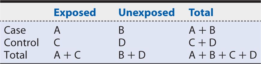
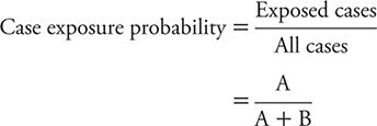
We begin by considering the exposure probability among cases, or the proportion of cases who were exposed previously. Using the notation introduced in Table 9-1, we calculate this probability as:
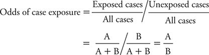
The odds of a case being exposed are estimated by the probability of a case being exposed divided by the probability of a case being unexposed. This measure is calculated as:
Using a comparable calculation, the odds of exposure among controls can be shown to be estimated by:
![]()
The ratio of these two odds (odds of exposure among cases divided by odds of exposure among controls) is referred to as the odds ratio (OR). The OR is calculated as:
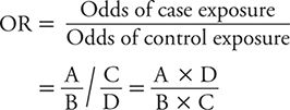
When newly diagnosed (incident) cases are sampled from the same source population as controls, and sampling is independent of exposure history (all features of a well-designed case-control study), it can be shown that the OR gives an approximation to the incidence rate ratio. So, although the OR is a distinct measure of association and the preferred measure in a case-control study, it has an interpretation analogous to the rate ratio or risk ratio. The null value (no association) of the OR is 1. Values of the OR greater than 1 indicate a positive association between exposure and disease. Values of the OR below 1 indicate an inverse association between exposure and disease.
To illustrate the calculation of an OR, let us consider a case-control study of LBW and end-stage renal disease (ESRD) conducted by Lackland and colleagues (2000). The investigators identified patients with ESRD from a regional registry of all persons undergoing dialysis for chronic renal failure. The birth certificates of these individuals were then located through a search of vital records information. From the birth certificates, information was extracted on LBW and other characteristics. Two controls of the same sex and race were selected for each case from the next registered birth certificates, which were filed in order of receipt, thereby tightly linking the respective birthdates of cases and controls. For the purposes of analysis, birth weights were classified into five ordered categories, with LBW defined, following convention, as less than 2500 g. The middle birth weight category of 3000 to 3499 g chosen as the referent (unexposed) group. A summary of the data that were observed is shown in Table 9-2. The OR calculated from these data would be:
![]()
Table 9-2. Summary of data on the association of low birth weight (LBW) with end-stage renal disease (ESRD).
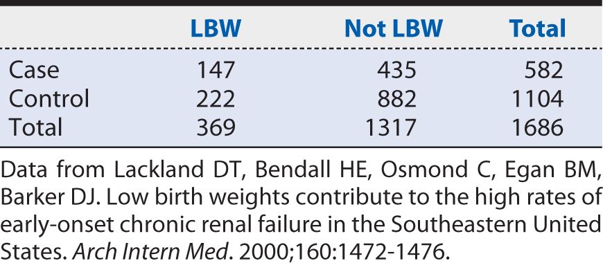
In other words, the odds of having been LBW were 34% higher among cases of ESRD than among controls. As with risk ratios, 95% confidence intervals (CIs) can be calculated around the point estimate of the OR. The approximate 95% CI for this OR is (1.06, 1.70). Because it excludes the null value (OR = 1), we can conclude that the observed association is unlikely to have arisen from chance alone. The strength of the association, as judged by the distance from the null value, nevertheless, may be characterized as relatively weak. As a rough guideline for interpretation, a moderate association would correspond to an OR approaching 2, and a relatively strong association would correspond to an OR of 3 or greater. These are somewhat subjective interpretations; however, a relatively weak strength of association may still have public health importance if the exposure is common and the disease involves appreciable morbidity and mortality.
Matching
A commonly used approach to selecting controls is to choose them in a direct pairing with individual cases. So, for example, we might choose for a white, male case who is age 65 years a white, male control of similar age (± a few years). We refer to this person-to-person alignment of cases and controls as matching. Another way of expressing this process is that controls are selected to parallel selected attributes of cases, such as demographic characteristics. The motivation for matching usually is to remove any disparity in these characteristics between the groups under comparison. There are two reasons for wanting to remove the influences of these other variables. The first is to reduce the potential for confounding. Confounding is a distorted exposure–disease association that is attributable in part or in whole to the influence of factors other than the exposure of interest. Confounding may be present when the persons who have the exposure of interest also have other risk factors that are less common in nonexposed persons. By matching, we remove any association of these matched factors with disease status (case vs. control) in the study population. This intent is achieved if matching is considered appropriately in the analysis.
A second motivation for matching is to obtain a more statistically precise estimate of effect, as might be reflected in narrower CIs around the point estimate. Again, this benefit requires an appropriate analysis for the matched design. From a purely pragmatic point of view, matching can help direct and simplify the process of selecting controls. For example, in the cited study of LBW and ESRD, after the cases were selected, a variety of methods could have been used to select controls, including using random digit telephone dialing, tax records, motor vehicle registrations, and so on. Because the information on LBW was going to be extracted from birth records, it made sense to use this source of information for selecting controls. By doing so, one could ensure that exposure information was available on controls and would be of similar quality and completeness to that of cases. The subjects were easily, quickly, and inexpensively sampled on the basis of sex, race, and date of birth. Here, then, the matching factors were three commonly used demographic characteristics. One often sees matching performed on the basis of these (or other) demographic attributes because often they are related to exposure likelihood as well as disease occurrence.
Matching can be performed on a one case-to-one control basis (pair matching). Alternatively, one often sees two, three, or more controls matched for each case. Enlarging the number of controls per case increases the statistical power of the study. This may be an important consideration for rare diseases where the number of eligible cases is limited. However, one reaches the point of diminishing returns in terms of statistical power by increasing the size of the control group. Typically, there is minimal gain in precision beyond a ratio of four controls per case. In the instance of the cited study of LBW and ESRD, for example, the matching ratio was two controls for every case.
It should be emphasized that the format for analysis described earlier and illustrated in Table 9-1 is for data in an unmatched study. If matching is performed, a slightly different tabular summary and analysis must be performed taking into account the matching in the design. The results of a matched and an unmatched analysis may give similar results, but this is not guaranteed, and the preferred approach on both validity and precision grounds is to consider the matching in the analysis. In fact, the analysis presented in Table 9-2 is an unmatched analysis and therefore not the preferred one for the manner in which the study was designed. As reported in the original publication, the analysis taking into account matching on sex, race and date of birth yielded an OR (95% CI) of 1.4 (1.1–1.8). The unmatched analysis yielded a similar but not identical OR of 1.3 (1.1–1.7). Such similarity is not a certainty, so ideally, the matched analysis is performed often using mathematical modeling to adjust for yet other factors. Mathematical modeling is beyond the scope of the present discussion. For those interested in conducting analyses of matched or unmatched case-control studies, Epi Info, a free, easy-to-use software package that has been developed by the Centers for Disease Control and Prevention, is available at wwwn.cdc.gov/epiinfo.
SUMMARY
In this chapter, we introduced another important type of observational research design referred to as a case-control study. This type of research approach is particularly well suited to the study of rare diseases and those with long developmental (latent) periods. The case-control study begins with the sampling of cases (persons with the disease of interest). A comparison group (controls) without the disease of interest then is selected. Information on earlier exposure histories of both cases and controls then is collected and contrasted between cases and controls.
Cases often are sampled from one or more hospital or other clinical facilities (a hospital-based sample). In other settings, an attempt is made to identify all cases within a community, region, workforce, or other group (population-based sample). Whereas some sampling schemes limit eligibility to newly diagnosed (incident) cases, other studies allow already existing (prevalent) cases to be included. A clear definition of diagnostic criteria is essential in order to select affected subjects appropriately.
Controls are sampled from the same source population that gave rise to the cases. This can be accomplished through a variety of sampling strategies from the same community or other group in a population-based study. Alternatively, in a hospital-based study, the controls tend to be selected from the same clinical facilities used to identify cases. Sampling controls from a hospital or outpatient facility is logistically advantageous, but it could lead to distorted exposure patterns if the illnesses of controls are long standing. To minimize the risk of a distorted conclusion, general guidelines for selecting hospital-based controls include choosing them from among multiple diagnostic categories and focusing on acute conditions such as trauma, infectious diseases, or other short-term illnesses.
The collection of information on exposure often is done through questionnaires or interviews with patients. This is a simple and quick technique, but it may be adversely affected by the ability of subjects to recall historical exposures. Even more concerning is the possibility that cases will recall exposures differently from controls, thereby distorting the results observed. Other approaches to collecting information on exposure include extracting data from historical records or, when possible, to collect biological markers of exposure.
The analysis of a case-control study involves comparing the odds of exposure among cases to the odds of exposure among controls. This contrast typically is presented as an OR, and it has a scale of measurement analogous to that of a risk ratio or rate ratio, with the null value of 1 and risk increasing exposures having values greater than 1 and risk lowering exposures having values less than 1. The further the point estimate of the OR is from 1, the stronger the association. Statistical precision of the estimate is reflected in the width of CIs around the point estimate.
Matching is a strategy for sampling control subjects in which key attributes (e.g., age, race, and sex) are linked on a person-to-person basis between cases and controls. Matching can be done on a one-to-one basis (pair matched) or with two or more controls per case. There may be some gain in statistical power by increasing the number of controls per case, but there usually is a diminishing return beyond four controls per case. The intent of matching is to control the influence of the matching factors on any observed association between the exposure and disease (confounding), as well as to improve the statistical precision of the study. To achieve these benefits, the matched sampling needs to be accompanied by a matched analysis. Data analysis software for both matched and unmatched analyses are widely available and easily used.

1. In a case-control study, the individuals with the disease of interest are limited to those who are newly diagnosed. We may describe these cases as
A. hospital based.
B. prevalent.
C. incident.
D. population based.
E. none of the above.
2. In a hospital-based case-control study, which of the following guidelines may be useful in sampling controls?
A. Choose them from a single diagnostic category
B. Choose them from a variety of diagnostic groups
C. Choose them from chronic conditions
D. Choose them from acute conditions
E. A and C
F. B and D
3. In a case-control study, matching may be performed to select controls in order to
A. control confounding.
B. control selection bias.
C. improve statistical precision.
D. increase the strength of association.
E. A and C.
F. B and D.
4. In contrast to a prospective cohort study, a case-control design may be preferred for the study of
A. rare exposures.
B. rare diseases.
C. shorter latent periods.
D. long latent periods.
E. A and C.
F. B and D.
5. The preferred measure of association in a case-control study is the
A. risk ratio.
B. rate ratio.
C. odds ratio.
D. attributable risk.
E. attributable risk percent.
6. Increasing the number of controls per case in a case-control study tends to reach diminishing returns in terms of increasing statistical power beyond what ratio?
A. 0.5 controls per case
B. 1.0 control per case
C. 2.0 controls per case
D. 3.0 controls per case
E. 4.0 controls per case
7. Which of the following are potential limitations of the use of historical records to determine exposure status in a case-control study?
A. Incomplete information
B. Missing records
C. Inaccurate information
D. All of the above
8. In a case-control study, the exposure of interest appears to be occurring more frequently among controls than among case, and the results appear to be unlikely to have occurred by chance alone. The corresponding OR (95% CI) is most likely to be
A. 0.5 (0.1, 1.1).
B. 0.7 (0.5, 0.9).
C. 1.0 (0.5, 2.0).
D. 1.5 (1.1, 2.3).
E. 2.0 (0.9, 3.5).
9. In a case-control study, if cases have a greater propensity than controls to remember earlier exposure histories, the study findings may be subject to
A. recall bias.
B. selection bias.
C. confounding.
D. length-biased sampling.
E. lead time bias.
10. Which of the following study types generally is considered to be most susceptible to bias?
A. Randomized controlled trial
B. Prospective cohort study
C. Case-control study
D. A cross-over study
Stay updated, free articles. Join our Telegram channel

Full access? Get Clinical Tree


